GUDHI Python modules documentation

Data structures for cell complexes
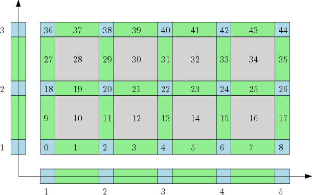
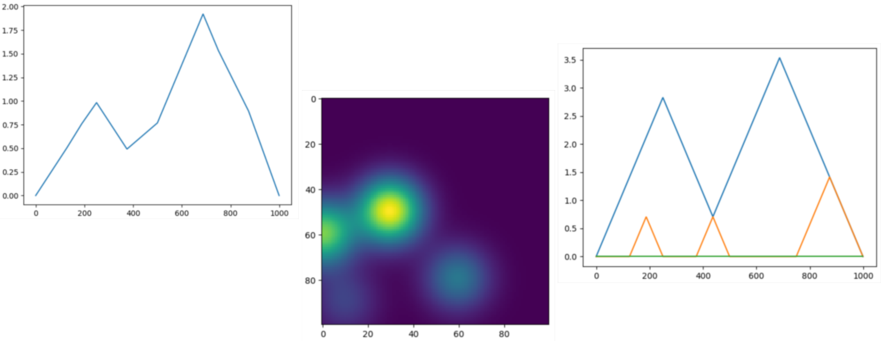
Cubical complexes
|
The cubical complex is an example of a structured complex useful in computational mathematics (specially rigorous numerics) and image analysis. |
|
Filtrations and reconstructions
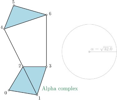
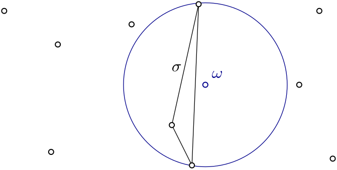
Alpha complex
|
Alpha complex is a simplicial complex constructed from the finite cells of a Delaunay Triangulation. The filtration value of each simplex is computed as the square of the circumradius of the simplex if the circumsphere is empty (the simplex is then said to be Gabriel), and as the minimum of the filtration values of the codimension 1 cofaces that make it not Gabriel otherwise. For performances reasons, it is advised to use CGAL ≥ 5.0.0. |
|
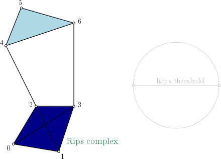
Rips complex
|
Rips complex is a simplicial complex constructed from a one skeleton graph. The filtration value of each edge is computed from a user-given distance function and is inserted until a user-given threshold value. This complex can be built from a point cloud and a distance function, or from a distance matrix. |
|
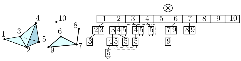
Witness complex
|
Witness complex \(Wit(W,L)\) is a simplicial complex defined on two sets of points in \(\mathbb{R}^D\). The data structure is described in [5]. |
|
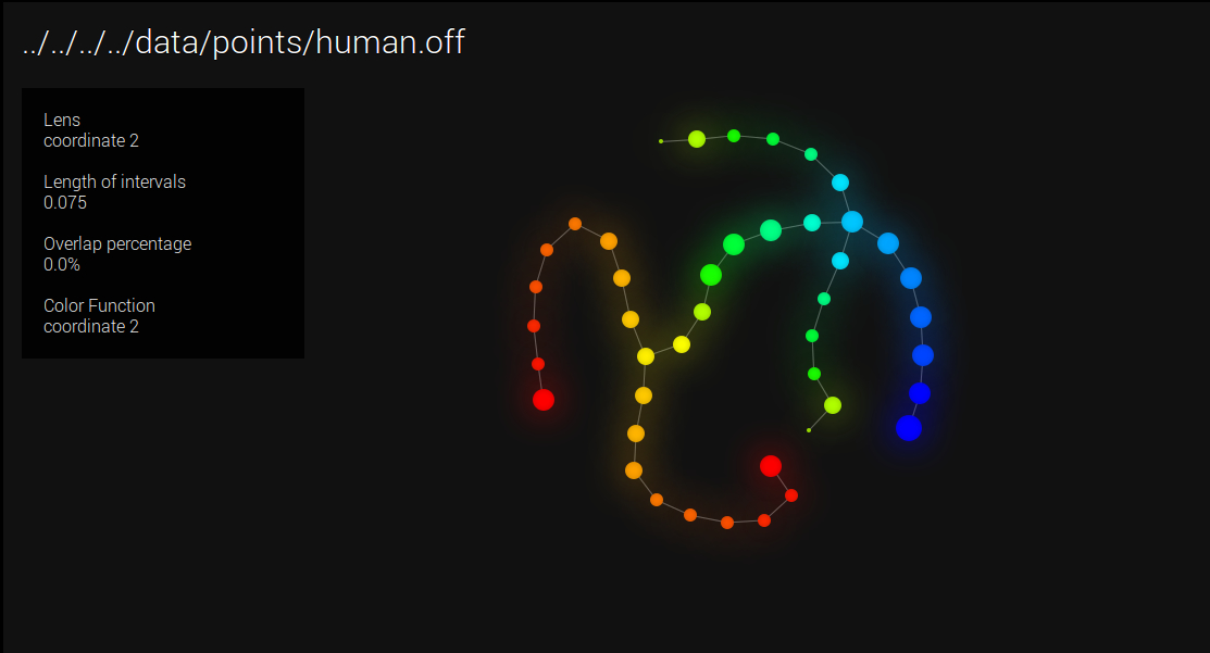
Cover complexes
|
Nerves and Graph Induced Complexes are cover complexes, i.e. simplicial complexes that provably contain topological information about the input data. They can be computed with a cover of the data, that comes i.e. from the preimage of a family of intervals covering the image of a scalar-valued function defined on the data. |
|
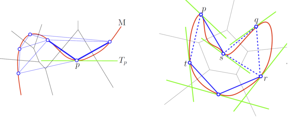
Tangential complex
|
A Tangential Delaunay complex is a simplicial complex designed to reconstruct a \(k\)-dimensional manifold embedded in \(d\)- dimensional Euclidean space. The input is a point sample coming from an unknown manifold. The running time depends only linearly on the extrinsic dimension \(d\) and exponentially on the intrinsic dimension \(k\). |
|
Topological descriptors computation
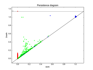
Persistence cohomology
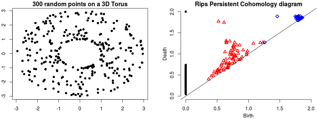
Rips Persistent Cohomology on a 3D Torus¶ |
The theory of homology consists in attaching to a topological space a sequence of (homology) groups, capturing global topological features like connected components, holes, cavities, etc. Persistent homology studies the evolution – birth, life and death – of these features when the topological space is changing. Consequently, the theory is essentially composed of three elements: topological spaces, their homology groups and an evolution scheme. Computation of persistent cohomology using the algorithm of [6] and [7] and the Compressed Annotation Matrix implementation of [8]. |
|
Please refer to each data structure that contains persistence feature for reference: |
||
Topological descriptors tools
Bottleneck distance
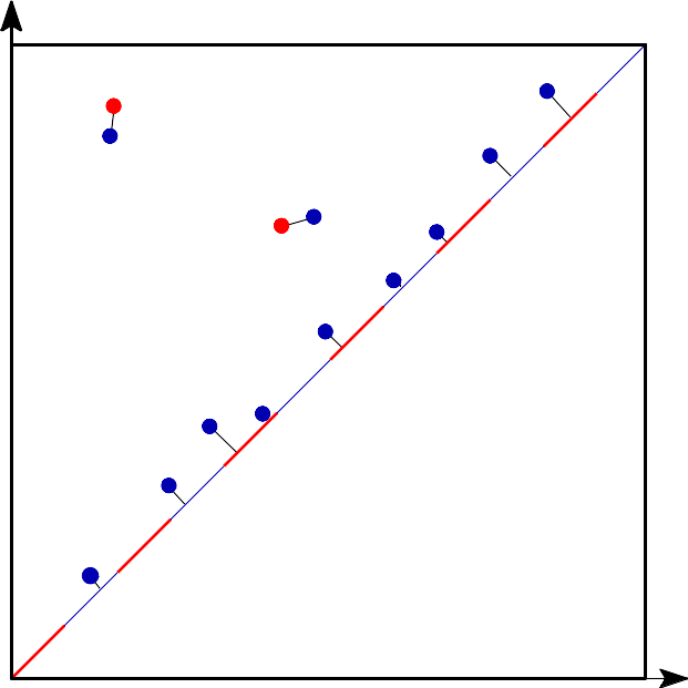
Bottleneck distance is the length of the longest edge¶ |
Bottleneck distance measures the similarity between two persistence diagrams. It’s the shortest distance b for which there exists a perfect matching between the points of the two diagrams (+ all the diagonal points) such that any couple of matched points are at distance at most b, where the distance between points is the sup norm in \(\mathbb{R}^2\). |
|
Wasserstein distance
|
Wasserstein distance is the q-th root of the sum of the edge lengths to the power q.¶ |
The q-Wasserstein distance measures the similarity between two persistence diagrams. It’s the minimum value c that can be achieved by a perfect matching between the points of the two diagrams (+ all diagonal points), where the value of a matching is defined as the q-th root of the sum of all edge lengths to the power q. Edge lengths are measured in norm p, for \(1 \leq p \leq \infty\). |
|
Persistence representations
|
Vectorizations, distances and kernels that work on persistence diagrams, compatible with scikit-learn. |
|
Persistence graphical tools
|
These graphical tools comes on top of persistence results and allows the user to build easily persistence barcode, diagram or density. |
|
Point cloud utilities
\((x_1, x_2, \ldots, x_d)\)
\((y_1, y_2, \ldots, y_d)\)
|
Utilities to process point clouds: read from file, subsample, etc. Parts of this package require CGAL. |
|
Bibliography
- 1
Alon Efrat, Alon Itai, and Matthew J. Katz. Geometry helps in bottleneck matching and related problems. Algorithmica, 31(1):1–28, 2001.
- 2
Michael Kerber, Dmitriy Morozov, and Arnur Nigmetov. Geometry helps to compare persistence diagrams. J. Exp. Algorithmics, 22:1.4:1–1.4:20, September 2017. URL: http://doi.acm.org/10.1145/3064175, doi:10.1145/3064175.
- 3
T. Kaczynski, K. Mischaikow, and M. Mrozek. Computational Homology. Applied Mathematical Sciences. Springer New York, 2004. ISBN 9780387408538. URL: https://books.google.fr/books?id=AShKtpi3GecC.
- 4
Hubert Wagner, Chao Chen, and Erald Vucini. Efficient Computation of Persistent Homology for Cubical Data, pages 91–106. Mathematics and Visualization. Springer Berlin Heidelberg, 2012. URL: http://dx.doi.org/10.1007/978-3-642-23175-9_7, doi:10.1007/978-3-642-23175-9_7.
- 5(1,2)
Jean-Daniel Boissonnat and Clément Maria. The simplex tree: an efficient data structure for general simplicial complexes. Algorithmica, pages 1–22, 2014. URL: http://dx.doi.org/10.1007/s00453-014-9887-3, doi:10.1007/s00453-014-9887-3.
- 6
Vin de Silva, Dmitriy Morozov, and Mikael Vejdemo-Johansson. Persistent cohomology and circular coordinates. Discrete & Computational Geometry, 45(4):737–759, 2011.
- 7
Tamal K. Dey, Fengtao Fan, and Yusu Wang. Computing topological persistence for simplicial maps. CoRR, 2012.
- 8
Jean-Daniel Boissonnat, Tamal K. Dey, and Clément Maria. The compressed annotation matrix: an efficient data structure for computing persistent cohomology. In ESA, 695–706. 2013. URL: http://dx.doi.org/10.1007/978-3-642-40450-4_59, doi:10.1007/978-3-642-40450-4_59.