Tangential complex user manual¶

	A Tangential Delaunay complex is a simplicial complex designed to reconstruct a \(k\)-dimensional manifold embedded in \(d\)- dimensional Euclidean space. The input is a point sample coming from an unknown manifold. The running time depends only linearly on the extrinsic dimension \(d\) and exponentially on the intrinsic dimension \(k\).	Author Clément Jamin Introduced in GUDHI 2.0.0 Copyright MIT (GPL v3) Requires Eigen \(\geq\) 3.1.0 and CGAL \(\geq\) 4.11.0
Tangential complex user manual	Tangential complex reference manual

Definition¶

A Tangential Delaunay complex is a simplicial complex designed to reconstruct a \(k\)-dimensional smooth manifold embedded in \(d\)-dimensional Euclidean space. The input is a point sample coming from an unknown manifold, which means that the points lie close to a structure of “small” intrinsic dimension. The running time depends only linearly on the extrinsic dimension \(d\) and exponentially on the intrinsic dimension \(k\).

An extensive description of the Tangential complex can be found in [20].

What is a Tangential Complex?¶

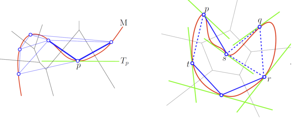
Let us start with the description of the Tangential complex of a simple example, with \(k = 1\) and \(d = 2\). The point set \(\mathscr P\) is located on a closed curve embedded in 2D. Only 4 points will be displayed (more are required for PCA) to simplify the figures.

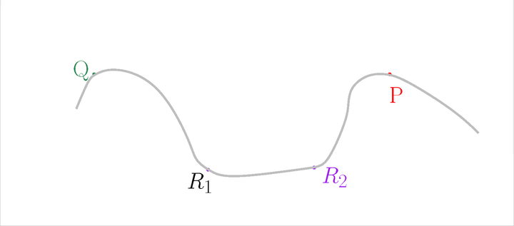
The input¶

For each point \(P\), estimate its tangent subspace \(T_P\) using PCA.

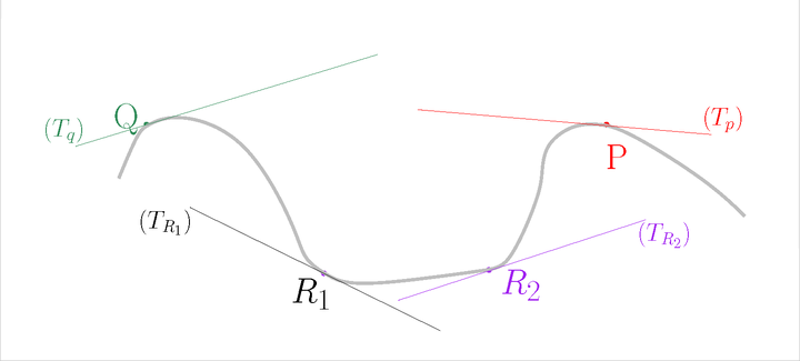
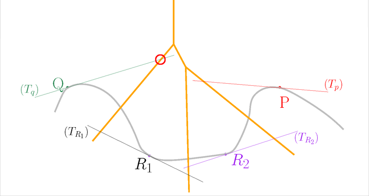
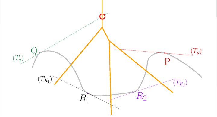
The estimated normals¶

Let us add the Voronoi diagram of the points in orange. For each point \(P\), construct its star in the Delaunay triangulation of \(\mathscr P\) restricted to \(T_P\).

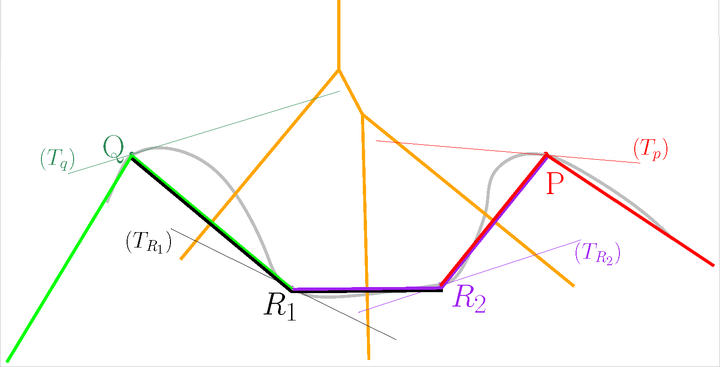
The Voronoi diagram¶

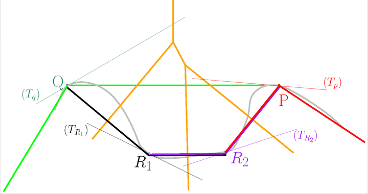
The Tangential Delaunay complex is the union of those stars.

In practice, neither the ambient Voronoi diagram nor the ambient Delaunay triangulation is computed. Instead, local \(k\)-dimensional regular triangulations are computed with a limited number of points as we only need the star of each point. More details can be found in [20].

Inconsistencies¶

Inconsistencies between the stars can occur. An inconsistency occurs when a simplex is not in the star of all its vertices.

Let us take the same example.

Before¶

Let us slightly move the tangent subspace \(T_Q\)

After¶

Now, the star of \(Q\) contains \(QP\), but the star of \(P\) does not contain \(QP\). We have an inconsistency.

After¶

One way to solve inconsistencies is to randomly perturb the positions of the points involved in an inconsistency. In the current implementation, this perturbation is done in the tangent subspace of each point. The maximum perturbation radius is given as a parameter to the constructor.

In most cases, we recommend to provide a point set where the minimum distance between any two points is not too small. This can be achieved using the functions provided by the Subsampling module. Then, a good value to start with for the maximum perturbation radius would be around half the minimum distance between any two points. The Example with perturbation below shows an example of such a process.

In most cases, this process is able to dramatically reduce the number of inconsistencies, but is not guaranteed to succeed.

Output¶

The result of the computation is exported as a SimplexTree. It is the union of the stars of all the input points. A vertex in the Simplex Tree is the index of the point in the range provided by the user. The point corresponding to a vertex can also be obtained through the gudhi.TangentialComplex.get_point() function. Note that even if the positions of the points are perturbed, their original positions are kept (e.g. get_point() returns the original position of the point).

The result can be obtained after the computation of the Tangential complex itself and/or after the perturbation process.

Simple example¶

This example builds the Tangential complex of point set read in an OFF file.

import gudhi
tc = gudhi.TangentialComplex(intrisic_dim = 1,
    off_file=gudhi.__root_source_dir__ + '/data/points/alphacomplexdoc.off')
tc.compute_tangential_complex()
result_str = 'Tangential contains ' + repr(tc.num_simplices()) + \
    ' simplices - ' + repr(tc.num_vertices()) + ' vertices.'
print(result_str)

st = tc.create_simplex_tree()
result_str = 'Simplex tree is of dimension ' + repr(st.dimension()) + \
    ' - ' + repr(st.num_simplices()) + ' simplices - ' + \
    repr(st.num_vertices()) + ' vertices.'
print(result_str)
for filtered_value in st.get_filtration():
    print(filtered_value[0])

The output is:

Tangential contains 12 simplices - 7 vertices.
Simplex tree is of dimension 1 - 15 simplices - 7 vertices.
[0]
[1]
[0, 1]
[2]
[0, 2]
[1, 2]
[3]
[1, 3]
[4]
[2, 4]
[5]
[4, 5]
[6]
[3, 6]
[5, 6]

Example with perturbation¶

This example builds the Tangential complex of a point set, then tries to solve inconsistencies by perturbing the positions of points involved in inconsistent simplices.

import gudhi
tc = gudhi.TangentialComplex(intrisic_dim = 1,
    points=[[0.0, 0.0], [1.0, 0.0], [0.0, 1.0], [1.0, 1.0]])
tc.compute_tangential_complex()
result_str = 'Tangential contains ' + repr(tc.num_vertices()) + ' vertices.'
print(result_str)

if tc.num_inconsistent_simplices() > 0:
    print('Tangential contains inconsistencies.')

tc.fix_inconsistencies_using_perturbation(10, 60)
if tc.num_inconsistent_simplices() == 0:
    print('Inconsistencies has been fixed.')

Bibliography

- 1
Alon Efrat, Alon Itai, and Matthew J. Katz. Geometry helps in bottleneck matching and related problems. Algorithmica, 31(1):1–28, 2001.
- 2
Michael Kerber, Dmitriy Morozov, and Arnur Nigmetov. Geometry helps to compare persistence diagrams. J. Exp. Algorithmics, 22:1.4:1–1.4:20, September 2017. URL: http://doi.acm.org/10.1145/3064175, doi:10.1145/3064175.
- 3
T. Kaczynski, K. Mischaikow, and M. Mrozek. Computational Homology. Applied Mathematical Sciences. Springer New York, 2004. ISBN 9780387408538. URL: https://books.google.fr/books?id=AShKtpi3GecC.
- 4
Hubert Wagner, Chao Chen, and Erald Vucini. Efficient Computation of Persistent Homology for Cubical Data, pages 91–106. Mathematics and Visualization. Springer Berlin Heidelberg, 2012. URL: http://dx.doi.org/10.1007/978-3-642-23175-9_7, doi:10.1007/978-3-642-23175-9_7.
- 5
Jean-Daniel Boissonnat and Clément Maria. The simplex tree: an efficient data structure for general simplicial complexes. Algorithmica, pages 1–22, 2014. URL: http://dx.doi.org/10.1007/s00453-014-9887-3, doi:10.1007/s00453-014-9887-3.
- 6
Vin de Silva, Dmitriy Morozov, and Mikael Vejdemo-Johansson. Persistent cohomology and circular coordinates. Discrete & Computational Geometry, 45(4):737–759, 2011.
- 7
Tamal K. Dey, Fengtao Fan, and Yusu Wang. Computing topological persistence for simplicial maps. CoRR, 2012.
- 8
Jean-Daniel Boissonnat, Tamal K. Dey, and Clément Maria. The compressed annotation matrix: an efficient data structure for computing persistent cohomology. In ESA, 695–706. 2013. URL: http://dx.doi.org/10.1007/978-3-642-40450-4_59, doi:10.1007/978-3-642-40450-4_59.
- 9
Mathieu Carrière, Bertrand Michel, and Steve Oudot. Statistical Analysis and Parameter Selection for Mapper. CoRR, 2017.
- 10
Tamal Dey, Fengtao Fan, and Yusu Wang. Graph induced complex on point data. In Proceedings of the Twenty-ninth Annual Symposium on Computational Geometry, 107–116. 2013.
- 11
Mathieu Carrière and Steve Oudot. Structure and Stability of the 1-Dimensional Mapper. CoRR, 2015.
- 12
James R. Munkres. Elements of algebraic topology. Addison-Wesley, 1984. ISBN 978-0-201-04586-4.
- 13
Herbert Edelsbrunner and John Harer. Computational Topology - an Introduction. American Mathematical Society, 2010. ISBN 978-0-8218-4925-5.
- 14
Afra Zomorodian and Gunnar E. Carlsson. Computing persistent homology. Discrete & Computational Geometry, 33(2):249–274, 2005.
- 15
Gunnar E. Carlsson and Vin de Silva. Zigzag persistence. Foundations of Computational Mathematics, 10(4):367–405, 2010.
- 16
Donald R. Sheehy. Linear-size approximations to the Vietoris-Rips filtration. Discrete & Computational Geometry, 49(4):778–796, 2013. doi:10.1007/s00454-013-9513-1.
- 17
Mickaël Buchet, Frédéric Chazal, Steve Y. Oudot, and Donald Sheehy. Efficient and robust persistent homology for measures. Computational Geometry: Theory and Applications, 58:70–96, 2016. doi:10.1016/j.comgeo.2016.07.001.
- 18
Nicholas J. Cavanna, Mahmoodreza Jahanseir, and Donald R. Sheehy. A geometric perspective on sparse filtrations. In Proceedings of the Canadian Conference on Computational Geometry. 2015. URL: http://research.cs.queensu.ca/cccg2015/CCCG15-papers/01.pdf.
- 19
Nicholas J. Cavanna, Mahmoodreza Jahanseir, and Donald R. Sheehy. Visualizing sparse filtrations. In Proceedings of the 31st International Symposium on Computational Geometry. 2015. doi:10.4230/LIPIcs.SOCG.2015.23.
- 20(1,2)
Jean-Daniel Boissonnat and Arijit Ghosh. Manifold reconstruction using tangential delaunay complexes. Discrete & Computational Geometry, 51(1):221–267, 2014. URL: http://dx.doi.org/10.1007/s00454-013-9557-2, doi:10.1007/s00454-013-9557-2.