Delaunay complex user manual#

Definition#

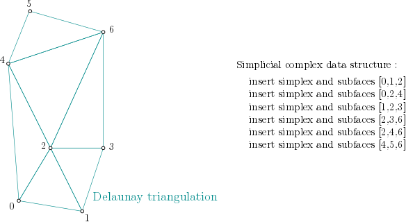
Delaunay complex is a simplicial complex constructed from the finite cells of a Delaunay Triangulation. The Simplicial complex filtration values can be computed with different filtrations (Delaunay complex, Delaunay Čech complex or Alpha complex)

When the simplicial complex filtration values are computed, it has the same persistent homology as the Čech complex, while being significantly smaller.

Author:: Vincent Rouvreau
Since:: GUDHI 2.0.0
License:: MIT (GPL v3)
Requires:: Eigen and CGAL

Delaunay complex user manual

Delaunay complex reference manual

DelaunayComplex is constructing a SimplexTree using Delaunay Triangulation [17] from the Computational Geometry Algorithms Library [32].

The Delaunay complex (all filtration values are set to NaN) is available by passing filtrations = None (default value) to create_simplex_tree().

When filtrations is:

‘alpha’ - The filtration value of each simplex is computed as an AlphaComplex
‘cech’ - The filtration value of each simplex is computed as a DelaunayCechComplex

Remarks about the `AlphaComplex` and the `DelaunayCechComplex`#

These remarks apply to the AlphaComplex and to the DelaunayCechComplex that we will call ‘complex’ in the following text.

When a complex is constructed with an infinite value of $α^{2}$ , the complex is a Delaunay complex (with special filtration values).
For people only interested in the topology of the complex (for instance persistence), notice the complex is equivalent to the Čech complex and much smaller if you do not bound the radii. Čech complex can still make sense in higher dimension precisely because you can bound the radii.
Using the default precision = 'safe' makes the construction safe, but, the filtration values are only guaranteed to have a small multiplicative error compared to the exact value, see set_float_relative_precision() to modify the precision. A drawback, when computing persistence, is that an empty exact interval [10^12,10^12] may become a non-empty approximate interval [10^12,10^12+10^6]. If you pass precision = 'exact' to the complex constructor, the filtration values are the exact ones converted to float. This can be very slow. Using precision = 'fast' makes the computations slightly faster, and the combinatorics are still exact, but the filtration values can exceptionally be arbitrarily bad. In all cases, we still guarantee that the output is a valid filtration (faces have a filtration value no larger than their cofaces).

DelaunayCechComplex is a bit faster than AlphaComplex, but only AlphaComplex has a weighted version.

Example from points#

This example builds the Delaunay Čech complex from the given points:

from gudhi import DelaunayCechComplex
points=[[1, 1], [7, 0], [4, 6], [9, 6], [0, 14], [2, 19], [9, 17]]
cpx = DelaunayCechComplex(points=points)

stree = cpx.create_simplex_tree(output_squared_values=False)
print(f"Complex is of dimension {stree.dimension()} - {stree.num_simplices()} simplices - ",
      f"{stree.num_vertices()} vertices.")
for filtered_value in stree.get_filtration():
    print("%s -> %.2f" % tuple(filtered_value))

The output is:

Complex is of dimension 2 - 25 simplices -  7 vertices.
[0] -> 0.00
[1] -> 0.00
[2] -> 0.00
[3] -> 0.00
[4] -> 0.00
[5] -> 0.00
[6] -> 0.00
[2, 3] -> 2.50
[4, 5] -> 2.69
[0, 2] -> 2.92
[0, 1] -> 3.04
[1, 3] -> 3.16
[1, 2] -> 3.35
[1, 2, 3] -> 3.54
[0, 1, 2] -> 3.60
[5, 6] -> 3.64
[2, 4] -> 4.47
[4, 6] -> 4.74
[4, 5, 6] -> 4.74
[3, 6] -> 5.50
[2, 6] -> 6.04
[2, 3, 6] -> 6.04
[2, 4, 6] -> 6.10
[0, 4] -> 6.52
[0, 2, 4] -> 6.52

Note: The Delaunay Čech complex can be easily replaced by the $α$ -complex, but note that the resulting filtration values will be different.

Weighted version#

A weighted version for $α$ -complex is available. It is like a usual $α$ -complex, but based on a CGAL regular triangulation.

In this case, the filtration value of each simplex is computed as the power distance of the smallest power sphere passing through all of its vertices. Weighted Alpha complex can have negative filtration values. If output_squared_values is set to False, filtration values will be NaN in this case.

This example builds the weighted $α$ -complex of a small molecule, where atoms have different sizes. It is taken from CGAL 3d weighted alpha shapes.

Then, it is asked to display information about the $α$ -complex.

from gudhi import AlphaComplex
wgt_ac = AlphaComplex(points=[[ 1., -1., -1.],
                              [-1.,  1., -1.],
                              [-1., -1.,  1.],
                              [ 1.,  1.,  1.],
                              [ 2.,  2.,  2.]],
                      weights = [4., 4., 4., 4., 1.])

stree = wgt_ac.create_simplex_tree(output_squared_values=True)
print(f"Weighted alpha is of dimension {stree.dimension()} - {stree.num_simplices()} simplices - ",
      f"{stree.num_vertices()} vertices.")
for simplex in stree.get_simplices():
    print("%s -> %.2f" % tuple(simplex))