Representations manual#

	Vectorizations, distances and kernels that work on persistence diagrams, compatible with scikit-learn and tensorflow.	Authors: Mathieu Carrière, Martin Royer, Gard Spreemann, Wojciech Reise Since: GUDHI 3.1.0 License: MIT
	Representations manual
	TensorFlow layer for representations

This module aims at bridging the gap between persistence diagrams and machine learning, by providing implementations of most of the vector representations for persistence diagrams in the literature, in a scikit-learn format. More specifically, it provides tools, using the scikit-learn standard interface, to compute distances and kernels on persistence diagrams, and to convert these diagrams into vectors in Euclidean space.

A diagram is represented as a numpy array of shape (n,2), as can be obtained from persistence_intervals_in_dimension() for instance. Points at infinity are represented as a numpy array of shape (n,1), storing only the birth time. The classes in this module can handle several persistence diagrams at once. In that case, the diagrams are provided as a list of numpy arrays. Note that it is not necessary for the diagrams to have the same number of points, i.e., for the corresponding arrays to have the same number of rows: all classes can handle arrays with different shapes.

This notebook explains how to efficiently combine machine learning and topological data analysis with the representations module in a scikit-learn fashion.

Examples#

Landscapes#

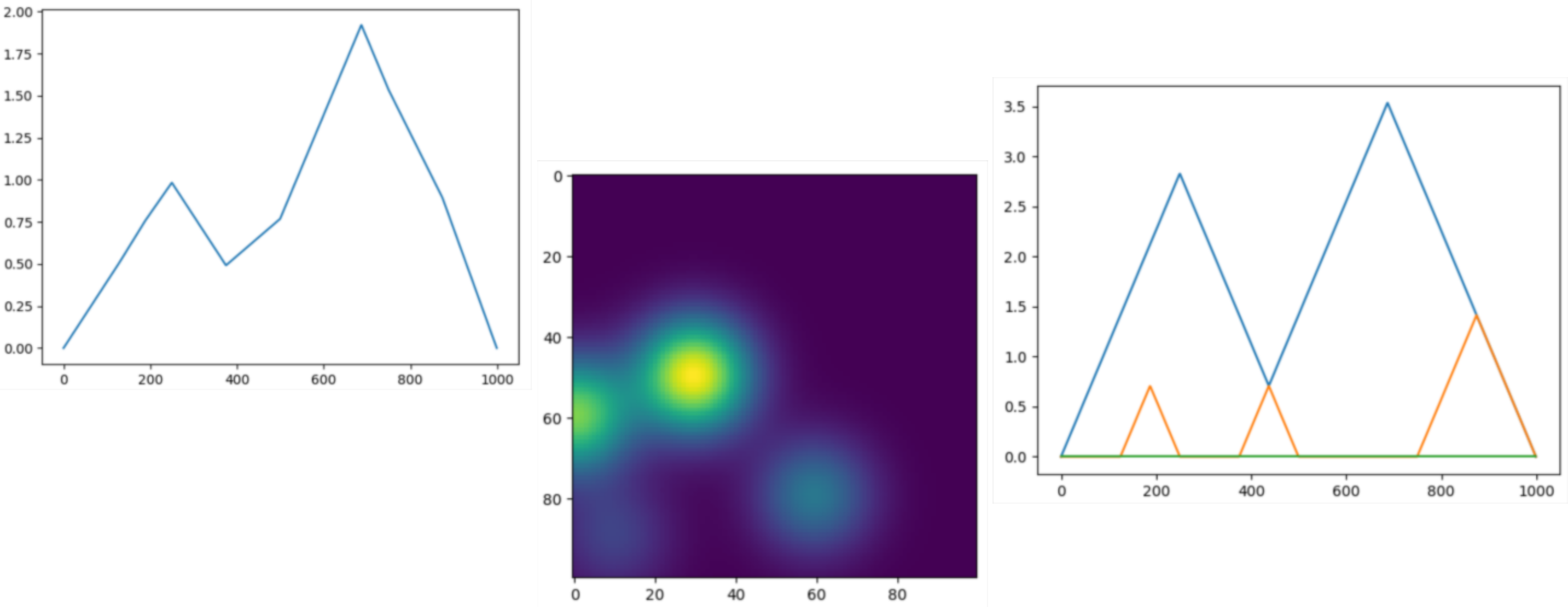
This example computes the first two Landscapes associated to a persistence diagram with four points. The landscapes are evaluated on ten samples, leading to two vectors with ten coordinates each, that are eventually concatenated in order to produce a single vector representation.

import numpy as np
from gudhi.representations import Landscape
# A single diagram with 4 points
D = np.array([[0.,4.],[1.,2.],[3.,8.],[6.,8.]])
diags = [D]
l=Landscape(num_landscapes=2,resolution=10).fit_transform(diags)
print(l)

[[1.02851895 2.05703791 2.57129739 1.54277843 0.89995409 1.92847304
95699199 3.08555686 2.05703791 1.02851895 0.         0.64282435
        0.         0.51425948 0.         0.         0.
77138922 1.02851895]]

Various kernels#

This small example is also provided diagram_vectorizations_distances_kernels.py

Utils#

class gudhi.representations.preprocessing.Clamping[source]#

Bases: BaseEstimator, TransformerMixin

This is a class for clamping a list of values. It is not meant to be called directly on (a list of) persistence diagrams, but it is rather meant to be used as a parameter for the DiagramScaler class. As such it has the same methods and purpose as common scalers from sklearn.preprocessing such as MinMaxScaler, RobustScaler, StandardScaler, etc. A typical use would be for instance if you want to clamp abscissae or ordinates (or both) of persistence diagrams within a pre-defined interval.

__init__(minimum=-inf, maximum=inf)[source]#

Constructor for the Clamping class.

Parameters:: limit¶ (float) – clamping value (default np.inf).

fit(X, y=None)[source]#

Fit the Clamping class on a list of values (this function actually does nothing but is useful when Clamping is included in a scikit-learn Pipeline).

Parameters:

X¶ (numpy array of size n) – input values.
y¶ (n x 1 array) – value labels (unused).

transform(X)[source]#

Clamp list of values.

Parameters:: X¶ (numpy array of size n) – input list of values.
Returns:: output list of values.
Return type:: numpy array of size n

Preprocessing#

class gudhi.representations.preprocessing.BirthPersistenceTransform[source]#

Bases: BaseEstimator, TransformerMixin

This is a class for the affine transformation (x,y) -> (x,y-x) to be applied on persistence diagrams.

__call__(diag)[source]#

Apply BirthPersistenceTransform on a single persistence diagram and outputs the result.

Parameters:: diag¶ (n x 2 numpy array) – input persistence diagram.
Returns:: transformed persistence diagram.
Return type:: n x 2 numpy array

__init__()[source]#: Constructor for BirthPersistenceTransform class.

fit(X, y=None)[source]#

Fit the BirthPersistenceTransform class on a list of persistence diagrams (this function actually does nothing but is useful when BirthPersistenceTransform is included in a scikit-learn Pipeline).

Parameters:

X¶ (list of n x 2 numpy array) – input persistence diagrams.
y¶ (n x 1 array) – persistence diagram labels (unused).

transform(X)[source]#

Apply the BirthPersistenceTransform function on the persistence diagrams.

Parameters:: X¶ (list of n x 2 numpy array) – input persistence diagrams.
Returns:: transformed persistence diagrams.
Return type:: list of n x 2 numpy array

class gudhi.representations.preprocessing.DiagramScaler[source]#

Bases: BaseEstimator, TransformerMixin

This is a class for preprocessing persistence diagrams with a given list of scalers, such as those included in scikit-learn.

__call__(diag)[source]#

Apply DiagramScaler on a single persistence diagram and outputs the result. If fit() hasn’t been run, this uses fit_transform on a clone of the object and thus does not affect later calls.

Parameters:: diag¶ (n x 2 numpy array) – input persistence diagram.
Returns:: transformed persistence diagram.
Return type:: n x 2 numpy array

__init__(use=False, scalers=[])[source]#

Constructor for the DiagramScaler class.

Parameters:

use¶ (bool) – whether to use the class or not (default False).
scalers¶ (list of classes) – list of scalers to be fit on the persistence diagrams (default []). Each element of the list is a tuple with two elements: the first one is a list of coordinates, and the second one is a scaler (i.e. a class with fit() and transform() methods) that is going to be applied to these coordinates. Common scalers can be found in the scikit-learn library (such as MinMaxScaler for instance).

fit(X, y=None)[source]#

Fit the DiagramScaler class on a list of persistence diagrams: persistence diagrams are concatenated in a big numpy array, and scalers are fit (by calling their fit() method) on their corresponding coordinates in this big array.

Parameters:

X¶ (list of n x 2 or n x 1 numpy arrays) – input persistence diagrams.
y¶ (n x 1 array) – persistence diagram labels (unused).

transform(X)[source]#

Apply the DiagramScaler function on the persistence diagrams. The fitted scalers are applied (by calling their transform() method) to their corresponding coordinates in each persistence diagram individually.

Parameters:: X¶ (list of n x 2 or n x 1 numpy arrays) – input persistence diagrams.
Returns:: transformed persistence diagrams.
Return type:: list of n x 2 or n x 1 numpy arrays

class gudhi.representations.preprocessing.DiagramSelector[source]#

Bases: BaseEstimator, TransformerMixin

This is a class for extracting finite or essential points in persistence diagrams.

__call__(diag)[source]#

Apply DiagramSelector on a single persistence diagram and outputs the result.

Parameters:: diag¶ (n x 2 numpy array) – input persistence diagram.
Returns:: extracted persistence diagram.
Return type:: n x 2 numpy array

__init__(use=False, limit=inf, point_type='finite')[source]#

Constructor for the DiagramSelector class.

Parameters:

use¶ (bool) – whether to use the class or not (default False).
limit¶ (float) – second coordinate value that is the criterion for being an essential point (default numpy.inf).
point_type¶ (string) – either “finite” or “essential”. The type of the points that are going to be extracted.

fit(X, y=None)[source]#

Fit the DiagramSelector class on a list of persistence diagrams (this function actually does nothing but is useful when DiagramSelector is included in a scikit-learn Pipeline).

Parameters:

X¶ (list of n x 2 or n x 1 numpy arrays) – input persistence diagrams.
y¶ (n x 1 array) – persistence diagram labels (unused).

transform(X)[source]#

Extract and return the finite or essential points of each persistence diagram individually.

Parameters:: X¶ (list of n x 2 or n x 1 numpy arrays) – input persistence diagrams.
Returns:: extracted persistence diagrams.
Return type:: list of n x 2 or n x 1 numpy arrays

class gudhi.representations.preprocessing.DimensionSelector[source]#

Bases: BaseEstimator, TransformerMixin

This is a class to select persistence diagrams in a specific dimension from its index.

__init__(index=0)[source]#

Constructor for the DimensionSelector class.

Parameters:: index¶ (int) – The returned persistence diagrams dimension index. Default value is 0.

fit(X, Y=None)[source]#: Nothing to be done, but useful when included in a scikit-learn Pipeline.

transform(X, Y=None)[source]#

Select persistence diagrams from its dimension.

Parameters:: X¶ (list of list of tuple) – List of list of persistence pairs, i.e. [[array( Hi(X0) ), array( Hj(X0) ), …], [array( Hi(X1) ), array( Hj(X1) ), …], …]
Returns:: Persistence diagrams in a specific dimension. i.e. if index was set to m and Hn is at index m of the input, it returns [array( Hn(X0) ), array( Hn(X1), …]
Return type:: list of tuple

class gudhi.representations.preprocessing.Padding[source]#

Bases: BaseEstimator, TransformerMixin

This is a class for padding a list of persistence diagrams with dummy points, so that all persistence diagrams end up with the same number of points.

__call__(diag)[source]#

Apply Padding on a single persistence diagram and outputs the result. If fit() hasn’t been run, this uses fit_transform on a clone of the object and thus does not affect later calls.

Parameters:: diag¶ (n x 2 numpy array) – input persistence diagram.
Returns:: padded persistence diagram.
Return type:: n x 2 numpy array

__init__(use=False)[source]#

Constructor for the Padding class.

Parameters:: use¶ (bool) – whether to use the class or not (default False).

fit(X, y=None)[source]#

Fit the Padding class on a list of persistence diagrams.

Parameters:

X¶ (list of n x 2 or n x 1 numpy arrays) – input persistence diagrams.
y¶ (n x 1 array) – persistence diagram labels (unused).

transform(X)[source]#

Add dummy points to each persistence diagram so that they all have the same cardinality. All points are given an additional coordinate indicating if the point was added after padding (0) or already present before (1).

Parameters:: X¶ (list of n x 2 or n x 1 numpy arrays) – input persistence diagrams.
Returns:: padded persistence diagrams.
Return type:: list of n x 3 or n x 2 numpy arrays

class gudhi.representations.preprocessing.ProminentPoints[source]#

Bases: BaseEstimator, TransformerMixin

This is a class for removing points that are close or far from the diagonal in persistence diagrams. If persistence diagrams are n x 2 numpy arrays (i.e. persistence diagrams with ordinary features), points are ordered and thresholded by distance-to-diagonal. If persistence diagrams are n x 1 numpy arrays (i.e. persistence diagrams with essential features), points are not ordered and thresholded by first coordinate.

__call__(diag)[source]#

Apply ProminentPoints on a single persistence diagram and outputs the result.

Parameters:: diag¶ (n x 2 numpy array) – input persistence diagram.
Returns:: thresholded persistence diagram.
Return type:: n x 2 numpy array

__init__(use=False, num_pts=10, threshold=-1, location='upper')[source]#

Constructor for the ProminentPoints class.

Parameters:

use¶ (bool) – whether to use the class or not (default False).
location¶ (string) – either “upper” or “lower” (default “upper”). Whether to keep the points that are far away (“upper”) or close (“lower”) to the diagonal.
num_pts¶ (int) – cardinality threshold (default 10). If location == “upper”, keep the top num_pts points that are the farthest away from the diagonal. If location == “lower”, keep the top num_pts points that are the closest to the diagonal.
threshold¶ (float) – distance-to-diagonal threshold (default -1). If location == “upper”, keep the points that are at least at a distance threshold from the diagonal. If location == “lower”, keep the points that are at most at a distance threshold from the diagonal.

fit(X, y=None)[source]#

Fit the ProminentPoints class on a list of persistence diagrams (this function actually does nothing but is useful when ProminentPoints is included in a scikit-learn Pipeline).

Parameters:

X¶ (list of n x 2 or n x 1 numpy arrays) – input persistence diagrams.
y¶ (n x 1 array) – persistence diagram labels (unused).

transform(X)[source]#

If location == “upper”, first select the top num_pts points that are the farthest away from the diagonal, then select and return from these points the ones that are at least at distance threshold from the diagonal for each persistence diagram individually. If location == “lower”, first select the top num_pts points that are the closest to the diagonal, then select and return from these points the ones that are at most at distance threshold from the diagonal for each persistence diagram individually.

Parameters:: X¶ (list of n x 2 or n x 1 numpy arrays) – input persistence diagrams.
Returns:: thresholded persistence diagrams.
Return type:: list of n x 2 or n x 1 numpy arrays

Vector methods#

class gudhi.representations.vector_methods.Atol[source]#

Bases: BaseEstimator, TransformerMixin

This class allows to vectorise measures (e.g. point clouds, persistence diagrams, etc) after a quantisation step.

ATOL paper: [27]

Example

>>> from sklearn.cluster import KMeans
>>> from gudhi.representations.vector_methods import Atol
>>> import numpy as np
>>> a = np.array([[1, 2, 4], [1, 4, 0], [1, 0, 4]])
>>> b = np.array([[4, 2, 0], [4, 4, 0], [4, 0, 2]])
>>> c = np.array([[3, 2, -1], [1, 2, -1]])
>>> atol_vectoriser = Atol(quantiser=KMeans(n_clusters=2, random_state=202006, n_init=10))
>>> atol_vectoriser.fit(X=[a, b, c]).centers
array([[ 2.6       ,  2.8       , -0.4       ],
       [ 2.        ,  0.66666667,  3.33333333]])
>>> atol_vectoriser(a)
array([0.42375966, 1.18168665])
>>> atol_vectoriser(c)
array([1.25157463, 0.02062512])
>>> atol_vectoriser.transform(X=[a, b, c])
array([[0.42375966, 1.18168665],
       [1.06330156, 0.29861028],
       [1.25157463, 0.02062512]])

__call__(measure, sample_weight=None)[source]#

Apply measure vectorisation on a single measure. Only available after fit has been called.

Parameters:: measure¶ (n x d numpy array) – input measure in R^d.
Returns:: numpy array in R^self.quantiser.n_clusters.

__init__(quantiser=KMeans(n_clusters=2, n_init='auto'), weighting_method='cloud', contrast='gaussian')[source]#

Constructor for the Atol measure vectorisation class.

Parameters:

quantiser¶ (Object) – Object with fit (sklearn API consistent) and cluster_centers and n_clusters attributes, e.g. sklearn.cluster.KMeans. It will be fitted when the Atol object function fit is called. Users are encouraged to provide their own quantiser, and in particular increase the number of clusters.
weighting_method¶ (string) – constant generic function for weighting the measure points choose from {“cloud”, “iidproba”} (default: constant function, i.e. the measure is seen as a point cloud by default). This will have no impact if weights are provided along with measures all the way: fit and transform.
contrast¶ (string) – constant function for evaluating proximity of a measure with respect to centers choose from {“gaussian”, “laplacian”, “indicator”} (default: gaussian contrast function, see page 3 in the ATOL paper).

fit(X, y=None, sample_weight=None)[source]#

Calibration step: fit centers to the sample measures and derive inertias between centers.

Parameters:

X¶ (list N x d numpy arrays) – input measures in R^d from which to learn center locations and inertias (measures can have different N).
y¶ – Ignored, present for API consistency by convention.
sample_weight¶ (list of numpy arrays) – weights for each measure point in X, optional. If None, the object’s weighting_method will be used.

Returns:

self

set_fit_request(*, sample_weight: bool | None | str = '$UNCHANGED$') → Atol#

Request metadata passed to the fit method.

Note that this method is only relevant if enable_metadata_routing=True (see sklearn.set_config()). Please see User Guide on how the routing mechanism works.

The options for each parameter are:

True: metadata is requested, and passed to fit if provided. The request is ignored if metadata is not provided.
False: metadata is not requested and the meta-estimator will not pass it to fit.
None: metadata is not requested, and the meta-estimator will raise an error if the user provides it.
str: metadata should be passed to the meta-estimator with this given alias instead of the original name.

The default (sklearn.utils.metadata_routing.UNCHANGED) retains the existing request. This allows you to change the request for some parameters and not others.

Added in version 1.3.

Note

This method is only relevant if this estimator is used as a sub-estimator of a meta-estimator, e.g. used inside a Pipeline. Otherwise it has no effect.

Parameters:: sample_weight¶ (str, True, False, or None, default=sklearn.utils.metadata_routing.UNCHANGED) – Metadata routing for sample_weight parameter in fit.
Returns:: self – The updated object.
Return type:: object

set_transform_request(*, sample_weight: bool | None | str = '$UNCHANGED$') → Atol#

Request metadata passed to the transform method.

Note that this method is only relevant if enable_metadata_routing=True (see sklearn.set_config()). Please see User Guide on how the routing mechanism works.

The options for each parameter are:

True: metadata is requested, and passed to transform if provided. The request is ignored if metadata is not provided.
False: metadata is not requested and the meta-estimator will not pass it to transform.
None: metadata is not requested, and the meta-estimator will raise an error if the user provides it.
str: metadata should be passed to the meta-estimator with this given alias instead of the original name.

The default (sklearn.utils.metadata_routing.UNCHANGED) retains the existing request. This allows you to change the request for some parameters and not others.

Added in version 1.3.

Note

This method is only relevant if this estimator is used as a sub-estimator of a meta-estimator, e.g. used inside a Pipeline. Otherwise it has no effect.

Parameters:: sample_weight¶ (str, True, False, or None, default=sklearn.utils.metadata_routing.UNCHANGED) – Metadata routing for sample_weight parameter in transform.
Returns:: self – The updated object.
Return type:: object

transform(X, sample_weight=None)[source]#

Apply measure vectorisation on a list of measures.

Parameters:

X¶ (list N x d numpy arrays) – input measures in R^d from which to learn center locations and inertias (measures can have different N).
sample_weight¶ (list of numpy arrays) – weights for each measure point in X, optional. If None, the object’s weighting_method will be used.

Returns:

numpy array with shape (number of measures) x (self.quantiser.n_clusters).

class gudhi.representations.vector_methods.BettiCurve[source]#

Bases: BaseEstimator, TransformerMixin

Compute Betti curves from persistence diagrams. There are several modes of operation: with a given resolution (with or without a sample_range), with a predefined grid, and with none of the previous. With a predefined grid, the class computes the Betti numbers at those grid points. Without a predefined grid, if the resolution is set to None, it can be fit to a list of persistence diagrams and produce a grid that consists of (at least) the filtration values at which at least one of those persistence diagrams changes Betti numbers, and then compute the Betti numbers at those grid points. In the latter mode, the exact Betti curve is computed for the entire real line. Otherwise, if the resolution is given, the Betti curve is obtained by sampling evenly using either the given sample_range or based on the persistence diagrams.

Examples

If pd is a persistence diagram and xs is a nonempty grid of finite values such that xs[0] >= pd.min(), then the results of:

>>> bc = BettiCurve(predefined_grid=xs) 
>>> result = bc(pd) 

and

>>> from scipy.interpolate import interp1d 
>>> bc = BettiCurve(resolution=None, predefined_grid=None) 
>>> bettis = bc.fit_transform([pd]) 
>>> interp = interp1d(bc.grid_, bettis[0, :], kind="previous", fill_value="extrapolate") 
>>> result = np.array(interp(xs), dtype=int) 

are the same.

grid_#

The grid on which the Betti numbers are computed. If predefined_grid was specified, grid_ will always be that grid, independently of data. If not and resolution is None, the grid is fitted to capture all filtration values at which the Betti numbers change.

Type:: 1d array

__call__(diag)[source]#: Shorthand for transform on a single persistence diagram. If fit() hasn’t been run, this uses fit_transform on a clone of the object and thus does not affect later calls.

__init__(resolution=100, sample_range=[nan, nan], predefined_grid=None, *, keep_endpoints=False)[source]#

Constructor for the BettiCurve class.

Parameters:

resolution¶ (int) – number of samples for the piecewise-constant function (default 100), or None for the exact curve.
sample_range¶ ([double, double]) – minimum and maximum of the piecewise-constant function domain, of the form [x_min, x_max] (default [numpy.nan, numpy.nan]). It is the interval on which samples will be drawn evenly. If one of the values is numpy.nan, it can be computed from the persistence diagrams with the fit() method.
predefined_grid¶ (1d array or None, default=None) – Predefined filtration grid points at which to compute the Betti curves. Must be strictly ordered. Infinities are ok. If None (default), and resolution is given, the grid will be uniform from x_min to x_max in ‘resolution’ steps, otherwise a grid will be computed that captures all changes in Betti numbers in the provided data.
keep_endpoints¶ (bool) – when computing sample_range (fixed resolution, no predefined_grid), use the exact extremities. This is mostly useful for plotting, the default is to use a slightly smaller range.

fit(X, y=None)[source]#

Fit the BettiCurve class on a list of persistence diagrams: if any of the values in sample_range is numpy.nan, replace it with the corresponding value computed on the given list of persistence diagrams. When no predefined grid is provided and resolution set to None, compute a filtration grid that captures all changes in Betti numbers for all the given persistence diagrams.

Parameters:

X¶ (list of 2d arrays) – Persistence diagrams.
y¶ (None) – Ignored.

fit_transform(X, y=None)[source]#: The result is the same as fit(X) followed by transform(X), but potentially faster.

transform(X)[source]#

Compute Betti curves.

Parameters:: X¶ (list of 2d arrays) – Persistence diagrams.
Returns:: Betti numbers of the given persistence diagrams at the grid points given in self.grid_
Return type:: len(X).len(self.grid_) array of ints

class gudhi.representations.vector_methods.ComplexPolynomial[source]#

Bases: BaseEstimator, TransformerMixin

This is a class for computing complex polynomials from a list of persistence diagrams. The persistence diagram points are seen as the roots of some complex polynomial, whose coefficients are returned in a complex vector. See https://link.springer.com/chapter/10.1007%2F978-3-319-23231-7_27 for more details.

__call__(diag)[source]#

Apply ComplexPolynomial on a single persistence diagram and outputs the result.

Parameters:: diag¶ (n x 2 numpy array) – input persistence diagram.
Returns:: output complex vector of coefficients.
Return type:: numpy array with shape (threshold)

__init__(polynomial_type='R', threshold=10)[source]#

Constructor for the ComplexPolynomial class.

Parameters:

polynomial_type¶ (char) – either “R”, “S” or “T” (default “R”). Type of complex polynomial that is going to be computed (explained in https://link.springer.com/chapter/10.1007%2F978-3-319-23231-7_27).
threshold¶ (int) – number of coefficients (default 10). This is the dimension of the complex vector of coefficients, i.e. the number of coefficients corresponding to the largest degree terms of the polynomial. If -1, this threshold is computed from the list of persistence diagrams by considering the one with the largest number of points and using the dimension of its corresponding complex vector of coefficients as threshold.

fit(X, y=None)[source]#

Fit the ComplexPolynomial class on a list of persistence diagrams (this function actually does nothing but is useful when ComplexPolynomial is included in a scikit-learn Pipeline).

Parameters:

X¶ (list of n x 2 or n x 1 numpy arrays) – input persistence diagrams.
y¶ (n x 1 array) – persistence diagram labels (unused).

transform(X)[source]#

Compute the complex vector of coefficients for each persistence diagram individually and concatenate the results.

Parameters:: X¶ (list of n x 2 numpy arrays) – input persistence diagrams.
Returns:: output complex vectors of coefficients.
Return type:: numpy array with shape (number of diagrams) x (threshold)

class gudhi.representations.vector_methods.Entropy[source]#

Bases: BaseEstimator, TransformerMixin

This is a class for computing persistence entropy. Persistence entropy is a statistic for persistence diagrams inspired from Shannon entropy. This statistic can also be used to compute a feature vector, called the entropy summary function. See https://arxiv.org/pdf/1803.08304.pdf for more details. Note that a previous implementation was contributed by Manuel Soriano-Trigueros.

grid_#

In vector mode, the grid on which the entropy summary function is computed.

Type:: 1d array

__call__(diag)[source]#

Apply Entropy on a single persistence diagram and outputs the result. If fit() hasn’t been run, this uses fit_transform on a clone of the object and thus does not affect later calls.

Parameters:: diag¶ (n x 2 numpy array) – input persistence diagram.
Returns:: output entropy.
Return type:: numpy array with shape (1 if mode = “scalar” else resolution)

__init__(mode='scalar', normalized=True, resolution=100, sample_range=[nan, nan], *, keep_endpoints=False)[source]#

Constructor for the Entropy class.

Parameters:

mode¶ (string) – what entropy to compute: either “scalar” for computing the entropy statistics, or “vector” for computing the entropy summary functions (default “scalar”).
normalized¶ (bool) – whether to normalize the entropy summary function (default True). Used only if mode = “vector”.
resolution¶ (int) – number of sample for the entropy summary function (default 100). Used only if mode = “vector”.
sample_range¶ ([double, double]) – minimum and maximum of the entropy summary function domain, of the form [x_min, x_max] (default [numpy.nan, numpy.nan]). It is the interval on which samples will be drawn evenly. If one of the values is numpy.nan, it can be computed from the persistence diagrams with the fit() method. Used only if mode = “vector”.
keep_endpoints¶ (bool) – when computing sample_range, use the exact extremities. This is mostly useful for plotting, the default is to use a slightly smaller range.

fit(X, y=None)[source]#

Fit the Entropy class on a list of persistence diagrams.

Parameters:

X¶ (list of n x 2 numpy arrays) – input persistence diagrams.
y¶ (n x 1 array) – persistence diagram labels (unused).

transform(X)[source]#

Compute the entropy for each persistence diagram individually and concatenate the results.

Parameters:: X¶ (list of n x 2 numpy arrays) – input persistence diagrams.
Returns:: output entropy.
Return type:: numpy array with shape (number of diagrams) x (1 if mode = “scalar” else resolution)

class gudhi.representations.vector_methods.Landscape[source]#

Bases: BaseEstimator, TransformerMixin

This is a class for computing persistence landscapes from a list of persistence diagrams. A persistence landscape is a collection of 1D piecewise-linear functions computed from the rank function associated to the persistence diagram. These piecewise-linear functions are then sampled evenly on a given range and the corresponding vectors of samples are concatenated and returned. See http://jmlr.org/papers/v16/bubenik15a.html for more details.

grid_#

The grid on which the landscapes are computed.

Type:: 1d array

__call__(diag)[source]#

Apply Landscape on a single persistence diagram and outputs the result. If fit() hasn’t been run, this uses fit_transform on a clone of the object and thus does not affect later calls.

Parameters:: diag¶ (n x 2 numpy array) – input persistence diagram.
Returns:: output persistence landscape.
Return type:: numpy array with shape (number of samples = num_landscapes x resolution)

__init__(num_landscapes=5, resolution=100, sample_range=[nan, nan], *, keep_endpoints=False)[source]#

Constructor for the Landscape class.

Parameters:

num_landscapes¶ (int) – number of piecewise-linear functions to output (default 5).
resolution¶ (int) – number of sample for all piecewise-linear functions (default 100).
sample_range¶ ([double, double]) – minimum and maximum of all piecewise-linear function domains, of the form [x_min, x_max] (default [numpy.nan, numpy.nan]). It is the interval on which samples will be drawn evenly. If one of the values is numpy.nan, it can be computed from the persistence diagrams with the fit() method.
keep_endpoints¶ (bool) – when computing sample_range, use the exact extremities (where the value is always 0). This is mostly useful for plotting, the default is to use a slightly smaller range.

fit(X, y=None)[source]#

Fit the Landscape class on a list of persistence diagrams: if any of the values in sample_range is numpy.nan, replace it with the corresponding value computed on the given list of persistence diagrams.

Parameters:

X¶ (list of n x 2 numpy arrays) – input persistence diagrams.
y¶ (n x 1 array) – persistence diagram labels (unused).

transform(X)[source]#

Compute the persistence landscape for each persistence diagram individually and concatenate the results.

Parameters:: X¶ (list of n x 2 numpy arrays) – input persistence diagrams.
Returns:: output persistence landscapes.
Return type:: numpy array with shape (number of diagrams) x (number of samples = num_landscapes x resolution)

class gudhi.representations.vector_methods.PersistenceImage[source]#

Bases: BaseEstimator, TransformerMixin

This is a class for computing persistence images from a list of persistence diagrams. A persistence image is a 2D function computed from a persistence diagram by convolving the diagram points with a weighted Gaussian kernel. The plane is then discretized into an image with pixels, which is flattened and returned as a vector. See http://jmlr.org/papers/v18/16-337.html for more details.

__call__(diag)[source]#

Apply PersistenceImage on a single persistence diagram and outputs the result. If fit() hasn’t been run, this uses fit_transform on a clone of the object and thus does not affect later calls.

Parameters:: diag¶ (n x 2 numpy array) – input persistence diagram.
Returns:: numpy array with shape (number of pixels = resolution[0] x resolution[1]):: output persistence image.

__init__(bandwidth=1.0, weight=<function PersistenceImage.<lambda>>, resolution=[20, 20], im_range=[nan, nan, nan, nan])[source]#

Constructor for the PersistenceImage class.

Parameters:

bandwidth¶ (double) – bandwidth of the Gaussian kernel (default 1.).
weight¶ (function) – weight function for the persistence diagram points (default constant function, ie lambda x: 1). This function must be defined on 2D points, ie lists or numpy arrays of the form [p_x,p_y].
resolution¶ ([int,int]) – size (in pixels) of the persistence image (default [20,20]).
im_range¶ ([double,double,double,double]) – minimum and maximum of each axis of the persistence image, of the form [x_min, x_max, y_min, y_max] (default [numpy.nan, numpy.nan, numpy.nan, numpyp.nan]). If one of the values is numpy.nan, it can be computed from the persistence diagrams with the fit() method.

fit(X, y=None)[source]#

Fit the PersistenceImage class on a list of persistence diagrams: if any of the values in im_range is numpy.nan, replace it with the corresponding value computed on the given list of persistence diagrams.

Parameters:

X¶ (list of n x 2 numpy arrays) – input persistence diagrams.
y¶ (n x 1 array) – persistence diagram labels (unused).

transform(X)[source]#

Compute the persistence image for each persistence diagram individually and store the results in a single numpy array.

Parameters:: X¶ (list of n x 2 numpy arrays) – input persistence diagrams.
Returns:: output persistence images.
Return type:: numpy array with shape (number of diagrams) x (number of pixels = resolution[0] x resolution[1])

class gudhi.representations.vector_methods.Silhouette[source]#

Bases: BaseEstimator, TransformerMixin

This is a class for computing persistence silhouettes from a list of persistence diagrams. A persistence silhouette is computed by taking a weighted average of the collection of 1D piecewise-linear functions given by the persistence landscapes, and then by evenly sampling this average on a given range. Finally, the corresponding vector of samples is returned. See https://arxiv.org/abs/1312.0308 for more details.

grid_#

The grid on which the silhouette is computed.

Type:: 1d array

__call__(diag)[source]#

Apply Silhouette on a single persistence diagram and outputs the result. If fit() hasn’t been run, this uses fit_transform on a clone of the object and thus does not affect later calls.

Parameters:: diag¶ (n x 2 numpy array) – input persistence diagram.
Returns:: output persistence silhouette.
Return type:: numpy array with shape (resolution)

__init__(weight=<function Silhouette.<lambda>>, resolution=100, sample_range=[nan, nan], *, keep_endpoints=False)[source]#

Constructor for the Silhouette class.

Parameters:

weight¶ (function) – weight function for the persistence diagram points (default constant function, ie lambda x: 1). This function must be defined on 2D points, ie on lists or numpy arrays of the form [p_x,p_y].
resolution¶ (int) – number of samples for the weighted average (default 100).
sample_range¶ ([double, double]) – minimum and maximum for the weighted average domain, of the form [x_min, x_max] (default [numpy.nan, numpy.nan]). It is the interval on which samples will be drawn evenly. If one of the values is numpy.nan, it can be computed from the persistence diagrams with the fit() method.
keep_endpoints¶ (bool) – when computing sample_range, use the exact extremities (where the value is always 0). This is mostly useful for plotting, the default is to use a slightly smaller range.

fit(X, y=None)[source]#

Fit the Silhouette class on a list of persistence diagrams: if any of the values in sample_range is numpy.nan, replace it with the corresponding value computed on the given list of persistence diagrams.

Parameters:

X¶ (list of n x 2 numpy arrays) – input persistence diagrams.
y¶ (n x 1 array) – persistence diagram labels (unused).

transform(X)[source]#

Compute the persistence silhouette for each persistence diagram individually and concatenate the results.

Parameters:: X¶ (list of n x 2 numpy arrays) – input persistence diagrams.
Returns:: output persistence silhouettes.
Return type:: numpy array with shape (number of diagrams) x (resolution)

class gudhi.representations.vector_methods.TopologicalVector[source]#

Bases: BaseEstimator, TransformerMixin

This is a class for computing topological vectors from a list of persistence diagrams. The topological vector associated to a persistence diagram is the sorted vector of a slight modification of the pairwise distances between the persistence diagram points. See https://diglib.eg.org/handle/10.1111/cgf12692 for more details.

__call__(diag)[source]#

Apply TopologicalVector on a single persistence diagram and outputs the result.

Parameters:: diag¶ (n x 2 numpy array) – input persistence diagram.
Returns:: output topological vector.
Return type:: numpy array with shape (threshold)

__init__(threshold=10)[source]#

Constructor for the TopologicalVector class.

Parameters:: threshold¶ (int) – number of distances to keep (default 10). This is the dimension of the topological vector. If -1, this threshold is computed from the list of persistence diagrams by considering the one with the largest number of points and using the dimension of its corresponding topological vector as threshold.

fit(X, y=None)[source]#

Fit the TopologicalVector class on a list of persistence diagrams (this function actually does nothing but is useful when TopologicalVector is included in a scikit-learn Pipeline).

Parameters:

X¶ (list of n x 2 or n x 1 numpy arrays) – input persistence diagrams.
y¶ (n x 1 array) – persistence diagram labels (unused).

transform(X)[source]#

Compute the topological vector for each persistence diagram individually and concatenate the results.

Parameters:: X¶ (list of n x 2 numpy arrays) – input persistence diagrams.
Returns:: output topological vectors.
Return type:: numpy array with shape (number of diagrams) x (threshold)

Kernel methods#

class gudhi.representations.kernel_methods.PersistenceFisherKernel[source]#

Bases: BaseEstimator, TransformerMixin

This is a class for computing the persistence Fisher kernel matrix from a list of persistence diagrams. The persistence Fisher kernel is computed by exponentiating the corresponding persistence Fisher distance with a Gaussian kernel. See papers.nips.cc/paper/8205-persistence-fisher-kernel-a-riemannian-manifold-kernel-for-persistence-diagrams for more details.

__call__(diag1, diag2)[source]#

Apply PersistenceFisherKernel on a single pair of persistence diagrams and outputs the result.

Parameters:

diag1¶ (n x 2 numpy array) – first input persistence diagram.
diag2¶ (n x 2 numpy array) – second input persistence diagram.

Returns:

persistence Fisher kernel value.

Return type:

float

__init__(bandwidth_fisher=1.0, bandwidth=1.0, kernel_approx=None, n_jobs=None)[source]#

Constructor for the PersistenceFisherKernel class.

Parameters:

bandwidth¶ (double) – bandwidth of the Gaussian kernel applied to the persistence Fisher distance (default 1.).
bandwidth_fisher¶ (double) – bandwidth of the Gaussian kernel used to turn persistence diagrams into probability distributions by PersistenceFisherDistance class (default 1.).
kernel_approx¶ (class) – kernel approximation class used to speed up computation (default None). Common kernel approximations classes can be found in the scikit-learn library (such as RBFSampler for instance).
n_jobs¶ (int) – number of jobs to use for the computation. See pairwise_persistence_diagram_kernels() for details.

fit(X, y=None)[source]#

Fit the PersistenceFisherKernel class on a list of persistence diagrams: an instance of the PersistenceFisherDistance class is fitted on the diagrams and then stored.

Parameters:

X¶ (list of n x 2 numpy arrays) – input persistence diagrams.
y¶ (n x 1 array) – persistence diagram labels (unused).

transform(X)[source]#

Compute all persistence Fisher kernel values between the persistence diagrams that were stored after calling the fit() method, and a given list of (possibly different) persistence diagrams.

Parameters:: X¶ (list of n x 2 numpy arrays) – input persistence diagrams.
Returns:: matrix of pairwise persistence Fisher kernel values.
Return type:: numpy array of shape (number of diagrams in X) x (number of diagrams in diagrams)

class gudhi.representations.kernel_methods.PersistenceScaleSpaceKernel[source]#

Bases: BaseEstimator, TransformerMixin

This is a class for computing the persistence scale space kernel matrix from a list of persistence diagrams. The persistence scale space kernel is computed by adding the symmetric to the diagonal of each point in each persistence diagram, with negative weight, and then convolving the points with a Gaussian kernel. See https://www.cv-foundation.org/openaccess/content_cvpr_2015/papers/Reininghaus_A_Stable_Multi-Scale_2015_CVPR_paper.pdf for more details.

__call__(diag1, diag2)[source]#

Apply PersistenceScaleSpaceKernel on a single pair of persistence diagrams and outputs the result.

Parameters:

diag1¶ (n x 2 numpy array) – first input persistence diagram.
diag2¶ (n x 2 numpy array) – second input persistence diagram.

Returns:

persistence scale space kernel value.

Return type:

float

__init__(bandwidth=1.0, kernel_approx=None, n_jobs=None)[source]#

Constructor for the PersistenceScaleSpaceKernel class.

Parameters:

bandwidth¶ (double) – bandwidth of the Gaussian kernel with which persistence diagrams will be convolved (default 1.)
kernel_approx¶ (class) – kernel approximation class used to speed up computation (default None). Common kernel approximations classes can be found in the scikit-learn library (such as RBFSampler for instance).
n_jobs¶ (int) – number of jobs to use for the computation. See pairwise_persistence_diagram_kernels() for details.

fit(X, y=None)[source]#

Fit the PersistenceScaleSpaceKernel class on a list of persistence diagrams: symmetric to the diagonal of all points are computed and an instance of the PersistenceWeightedGaussianKernel class is fitted on the diagrams and then stored.

Parameters:

X¶ (list of n x 2 numpy arrays) – input persistence diagrams.
y¶ (n x 1 array) – persistence diagram labels (unused).

transform(X)[source]#

Compute all persistence scale space kernel values between the persistence diagrams that were stored after calling the fit() method, and a given list of (possibly different) persistence diagrams.

Parameters:: X¶ (list of n x 2 numpy arrays) – input persistence diagrams.
Returns:: matrix of pairwise persistence scale space kernel values.
Return type:: numpy array of shape (number of diagrams in X) x (number of diagrams in diagrams)

class gudhi.representations.kernel_methods.PersistenceWeightedGaussianKernel[source]#

Bases: BaseEstimator, TransformerMixin

This is a class for computing the persistence weighted Gaussian kernel matrix from a list of persistence diagrams. The persistence weighted Gaussian kernel is computed by convolving the persistence diagram points with weighted Gaussian kernels. See http://proceedings.mlr.press/v48/kusano16.html for more details.

__call__(diag1, diag2)[source]#

Apply PersistenceWeightedGaussianKernel on a single pair of persistence diagrams and outputs the result.

Parameters:

diag1¶ (n x 2 numpy array) – first input persistence diagram.
diag2¶ (n x 2 numpy array) – second input persistence diagram.

Returns:

persistence weighted Gaussian kernel value.

Return type:

float

__init__(bandwidth=1.0, weight=<function PersistenceWeightedGaussianKernel.<lambda>>, kernel_approx=None, n_jobs=None)[source]#

Constructor for the PersistenceWeightedGaussianKernel class.

Parameters:

bandwidth¶ (double) – bandwidth of the Gaussian kernel with which persistence diagrams will be convolved (default 1.)
weight¶ (function) – weight function for the persistence diagram points (default constant function, ie lambda x: 1). This function must be defined on 2D points, ie lists or numpy arrays of the form [p_x,p_y].
kernel_approx¶ (class) – kernel approximation class used to speed up computation (default None). Common kernel approximations classes can be found in the scikit-learn library (such as RBFSampler for instance).
n_jobs¶ (int) – number of jobs to use for the computation. See pairwise_persistence_diagram_kernels() for details.

fit(X, y=None)[source]#

Fit the PersistenceWeightedGaussianKernel class on a list of persistence diagrams: persistence diagrams are stored in a numpy array called diagrams and the kernel approximation class (if not None) is applied on them.

Parameters:

X¶ (list of n x 2 numpy arrays) – input persistence diagrams.
y¶ (n x 1 array) – persistence diagram labels (unused).

transform(X)[source]#

Compute all persistence weighted Gaussian kernel values between the persistence diagrams that were stored after calling the fit() method, and a given list of (possibly different) persistence diagrams.

Parameters:: X¶ (list of n x 2 numpy arrays) – input persistence diagrams.
Returns:: matrix of pairwise persistence weighted Gaussian kernel values.
Return type:: numpy array of shape (number of diagrams in X) x (number of diagrams in diagrams)

class gudhi.representations.kernel_methods.SlicedWassersteinKernel[source]#

Bases: BaseEstimator, TransformerMixin

This is a class for computing the sliced Wasserstein kernel matrix from a list of persistence diagrams. The sliced Wasserstein kernel is computed by exponentiating the corresponding sliced Wasserstein distance with a Gaussian kernel. See http://proceedings.mlr.press/v70/carriere17a.html for more details.

__call__(diag1, diag2)[source]#

Apply SlicedWassersteinKernel on a single pair of persistence diagrams and outputs the result.

Parameters:

diag1¶ (n x 2 numpy array) – first input persistence diagram.
diag2¶ (n x 2 numpy array) – second input persistence diagram.

Returns:

sliced Wasserstein kernel value.

Return type:

float

__init__(num_directions=10, bandwidth=1.0, n_jobs=None)[source]#

Constructor for the SlicedWassersteinKernel class.

Parameters:

bandwidth¶ (double) – bandwidth of the Gaussian kernel applied to the sliced Wasserstein distance (default 1.).
num_directions¶ (int) – number of lines evenly sampled from [-pi/2,pi/2] in order to approximate and speed up the kernel computation (default 10).
n_jobs¶ (int) – number of jobs to use for the computation. See pairwise_persistence_diagram_kernels() for details.

fit(X, y=None)[source]#

Fit the SlicedWassersteinKernel class on a list of persistence diagrams: an instance of the SlicedWassersteinDistance class is fitted on the diagrams and then stored.

Parameters:

X¶ (list of n x 2 numpy arrays) – input persistence diagrams.
y¶ (n x 1 array) – persistence diagram labels (unused).

transform(X)[source]#

Compute all sliced Wasserstein kernel values between the persistence diagrams that were stored after calling the fit() method, and a given list of (possibly different) persistence diagrams.

Parameters:: X¶ (list of n x 2 numpy arrays) – input persistence diagrams.
Returns:: matrix of pairwise sliced Wasserstein kernel values.
Return type:: numpy array of shape (number of diagrams in X) x (number of diagrams in diagrams)

gudhi.representations.kernel_methods.pairwise_persistence_diagram_kernels(X, Y=None, kernel='sliced_wasserstein', n_jobs=None, **kwargs)[source]#

This function computes the kernel matrix between two lists of persistence diagrams given as numpy arrays of shape (nx2).

Parameters:

X¶ (list of n numpy arrays of shape (numx2)) – first list of persistence diagrams.
Y¶ (list of m numpy arrays of shape (numx2)) – second list of persistence diagrams (optional). If None, pairwise kernel values are computed from the first list only.
kernel¶ – kernel to use. It can be either a string (“sliced_wasserstein”, “persistence_scale_space”, “persistence_weighted_gaussian”, “persistence_fisher”) or a function taking two numpy arrays of shape (nx2) and (mx2) as inputs. If it is a function, make sure that it is symmetric.
n_jobs¶ (int) – number of jobs to use for the computation. This uses joblib.Parallel(prefer=”threads”), so kernels that do not release the GIL may not scale unless run inside a joblib.parallel_backend block.
**kwargs¶ – optional keyword parameters. Any further parameters are passed directly to the kernel function. See the docs of the various kernel classes in this module.

Returns:

kernel matrix.

Return type:

numpy array of shape (nxm)

Metrics#

class gudhi.representations.metrics.BottleneckDistance[source]#

Bases: BaseEstimator, TransformerMixin

This is a class for computing the bottleneck distance matrix from a list of persistence diagrams.

Requires:: CGAL

__call__(diag1, diag2)[source]#

Apply BottleneckDistance on a single pair of persistence diagrams and outputs the result.

Parameters:

diag1¶ (n x 2 numpy array) – first input persistence diagram.
diag2¶ (n x 2 numpy array) – second input persistence diagram.

Returns:

bottleneck distance.

Return type:

float

__init__(epsilon=None, n_jobs=None)[source]#

Constructor for the BottleneckDistance class.

Parameters:

epsilon¶ (double) – absolute (additive) error tolerated on the distance (default is the smallest positive float), see gudhi.bottleneck_distance().
n_jobs¶ (int) – number of jobs to use for the computation. See pairwise_persistence_diagram_distances() for details.

fit(X, y=None)[source]#

Fit the BottleneckDistance class on a list of persistence diagrams: persistence diagrams are stored in a numpy array called diagrams.

Parameters:

X¶ (list of n x 2 numpy arrays) – input persistence diagrams.
y¶ (n x 1 array) – persistence diagram labels (unused).

transform(X)[source]#

Compute all bottleneck distances between the persistence diagrams that were stored after calling the fit() method, and a given list of (possibly different) persistence diagrams.

Parameters:: X¶ (list of n x 2 numpy arrays) – input persistence diagrams.
Returns:: matrix of pairwise bottleneck distances.
Return type:: numpy array of shape (number of diagrams in diagrams) x (number of diagrams in X)

class gudhi.representations.metrics.PersistenceFisherDistance[source]#

Bases: BaseEstimator, TransformerMixin

This is a class for computing the persistence Fisher distance matrix from a list of persistence diagrams. The persistence Fisher distance is obtained by computing the original Fisher distance between the probability distributions associated to the persistence diagrams given by convolving them with a Gaussian kernel. See http://papers.nips.cc/paper/8205-persistence-fisher-kernel-a-riemannian-manifold-kernel-for-persistence-diagrams for more details.

__call__(diag1, diag2)[source]#

Apply PersistenceFisherDistance on a single pair of persistence diagrams and outputs the result.

Parameters:

diag1¶ (n x 2 numpy array) – first input persistence diagram.
diag2¶ (n x 2 numpy array) – second input persistence diagram.

Returns:

persistence Fisher distance.

Return type:

float

__init__(bandwidth=1.0, kernel_approx=None, n_jobs=None)[source]#

Constructor for the PersistenceFisherDistance class.

Parameters:

bandwidth¶ (double) – bandwidth of the Gaussian kernel used to turn persistence diagrams into probability distributions (default 1.).
kernel_approx¶ (class) – kernel approximation class used to speed up computation (default None). Common kernel approximations classes can be found in the scikit-learn library (such as RBFSampler for instance).
n_jobs¶ (int) – number of jobs to use for the computation. See pairwise_persistence_diagram_distances() for details.

fit(X, y=None)[source]#

Fit the PersistenceFisherDistance class on a list of persistence diagrams: persistence diagrams are stored in a numpy array called diagrams and the kernel approximation class (if not None) is applied on them.

Parameters:

X¶ (list of n x 2 numpy arrays) – input persistence diagrams.
y¶ (n x 1 array) – persistence diagram labels (unused).

transform(X)[source]#

Compute all persistence Fisher distances between the persistence diagrams that were stored after calling the fit() method, and a given list of (possibly different) persistence diagrams.

Parameters:: X¶ (list of n x 2 numpy arrays) – input persistence diagrams.
Returns:: matrix of pairwise persistence Fisher distances.
Return type:: numpy array of shape (number of diagrams in diagrams) x (number of diagrams in X)

class gudhi.representations.metrics.SlicedWassersteinDistance[source]#

Bases: BaseEstimator, TransformerMixin

This is a class for computing the sliced Wasserstein distance matrix from a list of persistence diagrams. The Sliced Wasserstein distance is computed by projecting the persistence diagrams onto lines, comparing the projections with the 1-norm, and finally integrating over all possible lines. See http://proceedings.mlr.press/v70/carriere17a.html for more details.

__call__(diag1, diag2)[source]#

Apply SlicedWassersteinDistance on a single pair of persistence diagrams and outputs the result.

Parameters:

diag1¶ (n x 2 numpy array) – first input persistence diagram.
diag2¶ (n x 2 numpy array) – second input persistence diagram.

Returns:

sliced Wasserstein distance.

Return type:

float

__init__(num_directions=10, n_jobs=None)[source]#

Constructor for the SlicedWassersteinDistance class.

Parameters:

num_directions¶ (int) – number of lines evenly sampled from [-pi/2,pi/2] in order to approximate and speed up the distance computation (default 10).
n_jobs¶ (int) – number of jobs to use for the computation. See pairwise_persistence_diagram_distances() for details.

fit(X, y=None)[source]#

Fit the SlicedWassersteinDistance class on a list of persistence diagrams: persistence diagrams are projected onto the different lines. The diagrams themselves and their projections are then stored in numpy arrays, called diagrams_ and approx_diag_.

Parameters:

X¶ (list of n x 2 numpy arrays) – input persistence diagrams.
y¶ (n x 1 array) – persistence diagram labels (unused).

transform(X)[source]#

Compute all sliced Wasserstein distances between the persistence diagrams that were stored after calling the fit() method, and a given list of (possibly different) persistence diagrams.

Parameters:: X¶ (list of n x 2 numpy arrays) – input persistence diagrams.
Returns:: matrix of pairwise sliced Wasserstein distances.
Return type:: numpy array of shape (number of diagrams in diagrams) x (number of diagrams in X)

class gudhi.representations.metrics.WassersteinDistance[source]#

Bases: BaseEstimator, TransformerMixin

This is a class for computing the Wasserstein distance matrix from a list of persistence diagrams.

__call__(diag1, diag2)[source]#

Apply WassersteinDistance on a single pair of persistence diagrams and outputs the result.

Parameters:

diag1¶ (n x 2 numpy array) – first input persistence diagram.
diag2¶ (n x 2 numpy array) – second input persistence diagram.

Returns:

Wasserstein distance.

Return type:

float

__init__(order=1, internal_p=inf, mode='hera', delta=0.01, n_jobs=None)[source]#

Constructor for the WassersteinDistance class.

Parameters:

order¶ (int) – exponent for Wasserstein, default value is 1., see gudhi.wasserstein.wasserstein_distance().
internal_p¶ (int) – ground metric on the (upper-half) plane (i.e. norm l_p in R^2), default value is np.inf, see gudhi.wasserstein.wasserstein_distance().
mode¶ (str) – method for computing Wasserstein distance. Either “pot” or “hera”. Default set to “hera”.
delta¶ (float) – relative error 1+delta. Used only if mode == “hera”.
n_jobs¶ (int) – number of jobs to use for the computation. See pairwise_persistence_diagram_distances() for details.

fit(X, y=None)[source]#

Fit the WassersteinDistance class on a list of persistence diagrams: persistence diagrams are stored in a numpy array called diagrams.

Parameters:

X¶ (list of n x 2 numpy arrays) – input persistence diagrams.
y¶ (n x 1 array) – persistence diagram labels (unused).

transform(X)[source]#

Compute all Wasserstein distances between the persistence diagrams that were stored after calling the fit() method, and a given list of (possibly different) persistence diagrams.

Parameters:: X¶ (list of n x 2 numpy arrays) – input persistence diagrams.
Returns:: matrix of pairwise Wasserstein distances.
Return type:: numpy array of shape (number of diagrams in diagrams) x (number of diagrams in X)

gudhi.representations.metrics.pairwise_persistence_diagram_distances(X, Y=None, metric='bottleneck', n_jobs=None, **kwargs)[source]#

This function computes the distance matrix between two lists of persistence diagrams given as numpy arrays of shape (nx2).

Parameters:

X¶ (list of n numpy arrays of shape (numx2)) – first list of persistence diagrams.
Y¶ (list of m numpy arrays of shape (numx2)) – second list of persistence diagrams (optional). If None, pairwise distances are computed from the first list only.
metric¶ – distance to use. It can be either a string (“sliced_wasserstein”, “wasserstein”, “hera_wasserstein” (Wasserstein distance computed with Hera—note that Hera is also used for the default option “wasserstein”), “pot_wasserstein” (Wasserstein distance computed with POT), “bottleneck”, “persistence_fisher”) or a function taking two numpy arrays of shape (nx2) and (mx2) as inputs. If it is a function, make sure that it is symmetric and that it outputs 0 if called on the same two arrays.
n_jobs¶ (int) –
number of jobs to use for the computation. This uses joblib.Parallel(prefer=”threads”), so metrics that do not release the GIL may not scale unless run inside a joblib.parallel_backend block.
**kwargs¶ – optional keyword parameters. Any further parameters are passed directly to the distance function. See the docs of the various distance classes in this module.

Returns:

distance matrix

Return type:

numpy array of shape (nxm)