
Cubical complex user manual#
Definition#
|
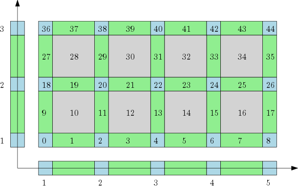
The cubical complex represents a grid as a cell complex with cells of all dimensions. |
|

|
||

|
||
The cubical complex is an example of a structured complex useful in computational mathematics (specially rigorous numerics) and image analysis.
An elementary interval is an interval of a form \([n,n+1]\), or \([n,n]\), for \(n \in \mathcal{Z}\). The first one is called non-degenerate, while the second one is a degenerate interval. A boundary of a elementary interval is a chain \(\partial [n,n+1] = [n+1,n+1]-[n,n]\) in case of non-degenerated elementary interval and \(\partial [n,n] = 0\) in case of degenerate elementary interval. An elementary cube \(C\) is a product of elementary intervals, \(C=I_1 \times \ldots \times I_n\). Embedding dimension of a cube is n, the number of elementary intervals (degenerate or not) in the product. A dimension of a cube \(C=I_1 \times ... \times I_n\) is the number of non degenerate elementary intervals in the product. A boundary of a cube \(C=I_1 \times \ldots \times I_n\) is a chain obtained in the following way:
(when working with a field of characteristic other than 2, the non-zero terms of this sum come with alternating signs ±1).
A cubical complex \(\mathcal{K}\) is a collection of cubes closed under operation of taking boundary (i.e. boundary of every cube from the collection is in the collection). A cube \(C\) in cubical complex \(\mathcal{K}\) is maximal if it is not in a boundary of any other cube in \(\mathcal{K}\). A support of a cube \(C\) is the set in \(\mathbb{R}^n\) occupied by \(C\) (\(n\) is the embedding dimension of \(C\)).
Cubes may be equipped with a filtration values in which case we have filtered cubical complex. All the cubical complexes considered in this implementation are filtered cubical complexes (although, the range of a filtration may be a set of two elements).
For further details and theory of cubical complexes, please consult [24] as well as the following paper [31].
Data structure#
The implementation of Cubical complex provides a representation of complexes that occupy a rectangular region in \(\mathbb{R}^n\). This extra assumption allows for a memory efficient way of storing cubical complexes in a form of so called bitmaps. Let \(R = [b_1,e_1] \times \ldots \times [b_n,e_n]\), for \(b_1,...b_n,e_1,...,e_n \in \mathbb{Z}\), \(b_i \leq d_i\) be the considered rectangular region and let \(\mathcal{K}\) be a filtered cubical complex having the rectangle \(R\) as its support. Note that the structure of the coordinate system gives a way a lexicographical ordering of cells of \(\mathcal{K}\). This ordering is a base of the presented bitmap-based implementation. In this implementation, the whole cubical complex is stored as a vector of the values of filtration. This, together with dimension of \(\mathcal{K}\) and the sizes of \(\mathcal{K}\) in all directions, allows to determine, dimension, neighborhood, boundary and coboundary of every cube \(C \in \mathcal{K}\).
Cubical complex.#
Note that the cubical complex in the figure above is, in a natural way, a product of one dimensional cubical complexes in \(\mathbb{R}\). The number of all cubes in each direction is equal \(2n+1\), where \(n\) is the number of maximal cubes in the considered direction. Let us consider a cube at the position \(k\) in the bitmap. Knowing the sizes of the bitmap, by a series of modulo operation, we can determine which elementary intervals are present in the product that gives the cube \(C\). In a similar way, we can compute boundary and the coboundary of each cube. Further details can be found in the literature.
Construction#
In the current implantation, filtration is given either at the maximal cubes or at the vertices, and it is then extended by the lower star filtration to all cubes. There are a number of constructors that can be used to construct cubical complex by users who want to use the code directly. They can be found in the Cubical complex reference manual.
from gudhi import CubicalComplex
import numpy as np
cc = CubicalComplex(top_dimensional_cells=np.array([[ 1.,  8.,  7.],
                                                    [ 4., 20.,  6.],
                                                    [ 6.,  4.,  5.]]))
print(f"Cubical complex is of dimension {cc.dimension()} - {cc.num_simplices()} simplices.")
the program output is:
Cubical complex is of dimension 2 - 49 simplices.
Periodic boundary conditions#
Often one would like to impose periodic boundary conditions to the cubical complex (cf. Periodic cubical complex reference manual). Let \(I_1\times ... \times I_n\) be a box that is decomposed with a cubical complex \(\mathcal{K}\). Imposing periodic boundary conditions in the direction i, means that the left and the right side of a complex \(\mathcal{K}\) are considered the same. In particular, if for a bitmap \(\mathcal{K}\) periodic boundary conditions are imposed in all directions, then complex \(\mathcal{K}\) became n-dimensional torus. One can use various constructors from the file Bitmap_cubical_complex_periodic_boundary_conditions_base.h to construct cubical complex with periodic boundary conditions.
It can be defined as follows:
from gudhi import PeriodicCubicalComplex as PCC
pcc = PCC(top_dimensional_cells = [[0, 0, 0], [0, 1, 0], [0, 0, 0]],
          periodic_dimensions=[True, False])
print(f"Periodic cubical complex is of dimension {pcc.dimension()} - {pcc.num_simplices()} simplices.")
the program output is:
Periodic cubical complex is of dimension 2 - 42 simplices.
Examples#
End user programs are available in python/example/ folder.
Tutorial#
This notebook explains how to represent sublevels sets of functions using cubical complexes.