GUDHI Python modules documentation

Data structures for cell complexes

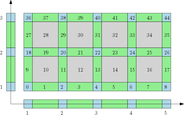
Cubical complexes

	The cubical complex represents a grid as a cell complex with cells of all dimensions.	Author Pawel Dlotko Since GUDHI 2.0.0 License MIT
Cubical complex user manual	Cubical complex reference manual Periodic cubical complex reference manual
	TensorFlow layer for cubical persistence	requires TensorFlow
	Cubical complex persistence scikit-learn like interface	Requires Scikit-learn

Simplicial complexes

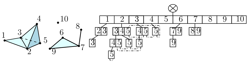
Simplex tree

	The simplex tree is an efficient and flexible data structure for representing general (filtered) simplicial complexes. The data structure is described in [5]	Author Clément Maria Since GUDHI 2.0.0 License MIT
Simplex tree user manual	Simplex tree reference manual
	TensorFlow layer for lower-star persistence on simplex trees	requires TensorFlow

Filtrations and reconstructions

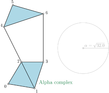
Alpha complex

	Alpha complex is a simplicial complex constructed from the finite cells of a Delaunay Triangulation. It has the same persistent homology as the Čech complex and is significantly smaller.	Author Vincent Rouvreau Since GUDHI 2.0.0 License MIT (GPL v3) Requires Eigen $\ge$ 3.1.0 and CGAL $\ge$ 5.1
Alpha complex user manual	Alpha complex reference manual

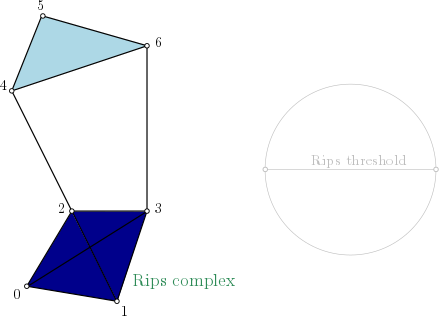
Rips complex

	The Vietoris-Rips complex is a simplicial complex built as the clique-complex of a proximity graph. We also provide sparse approximations, to speed-up the computation of persistent homology, and weighted versions, which are more robust to outliers.	Authors Clément Maria, Pawel Dlotko, Vincent Rouvreau, Marc Glisse, Yuichi Ike Since GUDHI 2.0.0 License MIT
Rips complex user manual	Rips complex reference manual
	TensorFlow layer for Vietoris-Rips persistence	requires TensorFlow

Witness complex

	Witness complex $Wit(W,L)$ is a simplicial complex defined on two sets of points in ${\mathbb{R}}^D$. The data structure is described in [5].	Author Siargey Kachanovich Since GUDHI 2.0.0 License MIT (GPL v3 for Euclidean versions only) Requires Eigen $\ge$ 3.1.0 and CGAL $\ge$ 4.11.0 for Euclidean versions only
Witness complex user manual	Witness complex reference manual Strong witness complex reference manual Euclidean witness complex reference manual Euclidean strong witness complex reference manual

Cover complexes

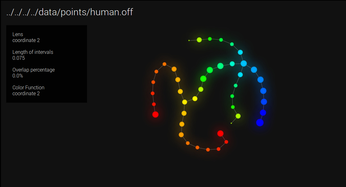
	Nerves and Graph Induced Complexes are cover complexes, i.e. simplicial complexes that provably contain topological information about the input data. They can be computed with a cover of the data, that comes i.e. from the preimage of a family of intervals covering the image of a scalar-valued function defined on the data.	Author Mathieu Carrière Since GUDHI 2.3.0 License MIT (GPL v3) Requires CGAL $\ge$ 4.11.0
Cover complexes user manual	Cover complexes reference manual

Tangential complex

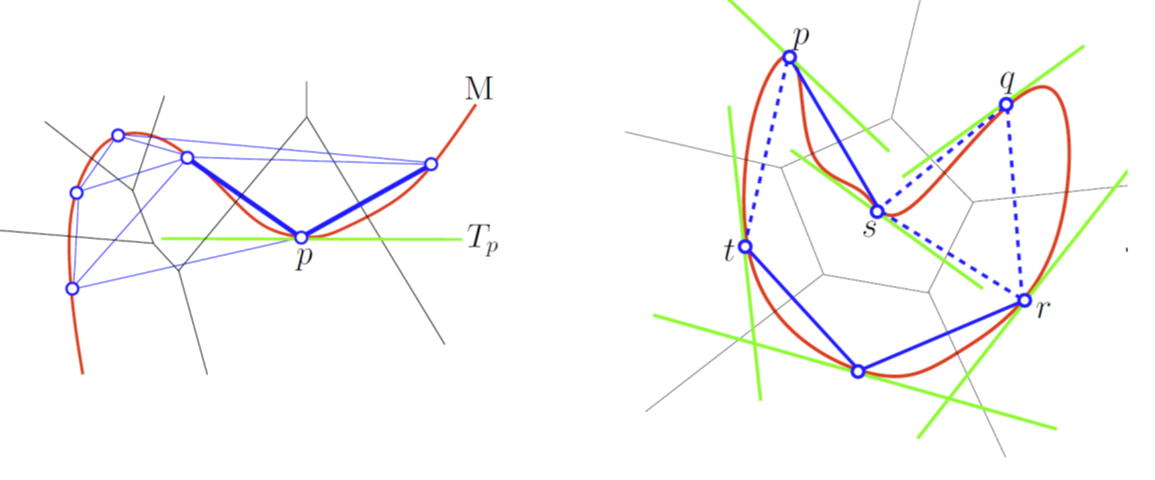
	A Tangential Delaunay complex is a simplicial complex designed to reconstruct a $k$-dimensional manifold embedded in $d$-dimensional Euclidean space. The input is a point sample coming from an unknown manifold. The running time depends only linearly on the extrinsic dimension $d$ and exponentially on the intrinsic dimension $k$.	Author Clément Jamin Since GUDHI 2.0.0 License MIT (GPL v3) Requires Eigen $\ge$ 3.1.0 and CGAL $\ge$ 4.11.0
Tangential complex user manual	Tangential complex reference manual

Topological descriptors computation

Persistent cohomology

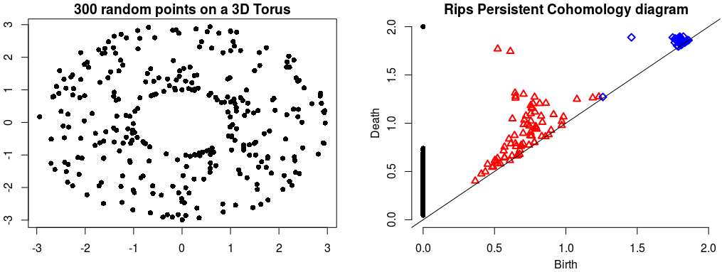
Rips Persistent Cohomology on a 3D Torus	The theory of homology consists in attaching to a topological space a sequence of (homology) groups, capturing global topological features like connected components, holes, cavities, etc. Persistent homology studies the evolution – birth, life and death – of these features when the topological space is changing. Computation of persistent cohomology using the algorithm of [15] and [18] and the Compressed Annotation Matrix implementation of [3].	Author Clément Maria Since GUDHI 2.0.0 License MIT
Persistent cohomology user manual	Please refer to each data structure that contains persistence feature for reference: Simplex tree reference manual Cubical complex reference manual Periodic cubical complex reference manual

Topological descriptors tools

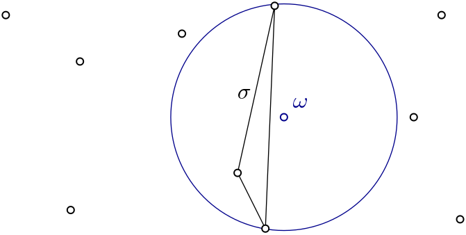
Bottleneck distance

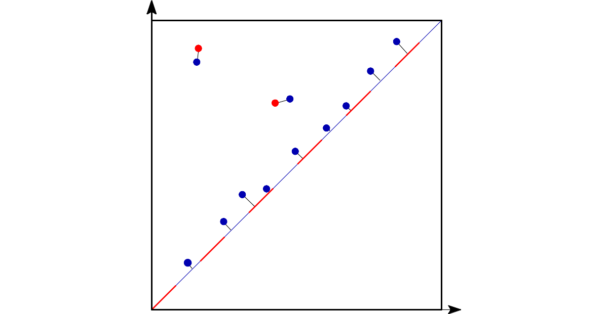
Bottleneck distance is the length of the longest edge	Bottleneck distance measures the similarity between two persistence diagrams. It’s the shortest distance b for which there exists a perfect matching between the points of the two diagrams (+ all the diagonal points) such that any couple of matched points are at distance at most b, where the distance between points is the sup norm in ${\mathbb{R}}^2$.	Author François Godi Since GUDHI 2.0.0 License MIT (GPL v3) Requires CGAL $\ge$ 4.11.0
Bottleneck distance user manual

Wasserstein distance

	The q-Wasserstein distance measures the similarity between two persistence diagrams using the sum of all edges lengths (instead of the maximum). It allows to define sophisticated objects such as barycenters of a family of persistence diagrams.	Author Theo Lacombe, Marc Glisse Since GUDHI 3.1.0 License MIT, BSD-3-Clause
Wasserstein distance user manual

Persistence representations

	Vectorizations, distances and kernels that work on persistence diagrams, compatible with scikit-learn.	Author Mathieu Carrière, Martin Royer Since GUDHI 3.1.0 License MIT Requires Scikit-learn
Representations manual

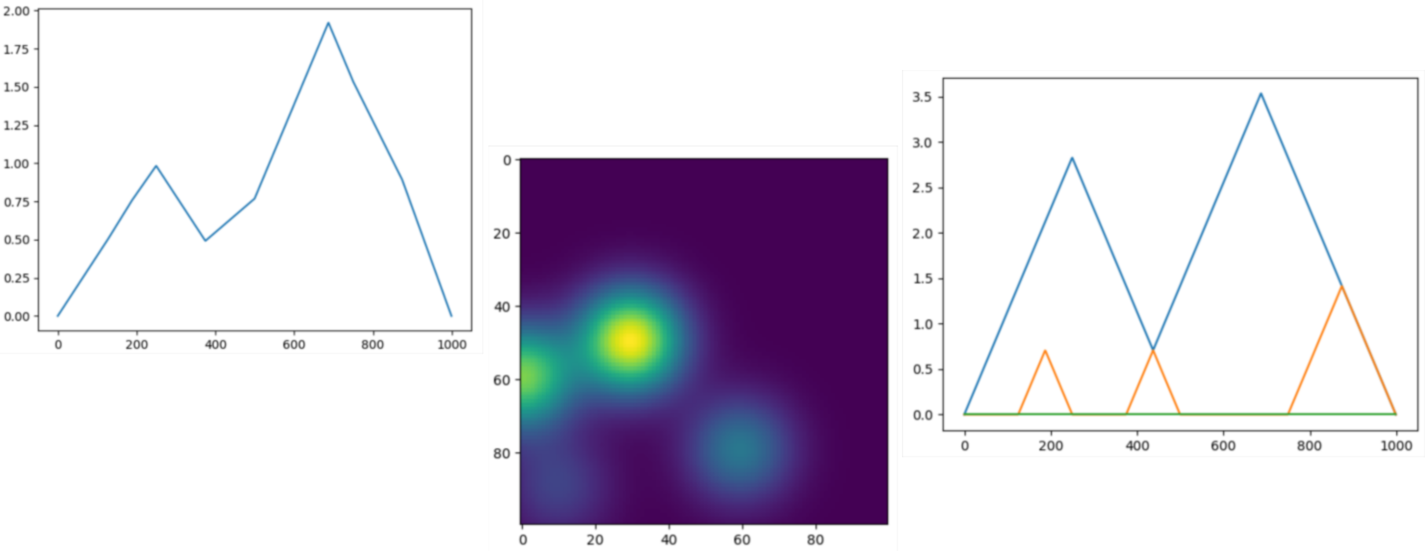
Persistence graphical tools

	These graphical tools comes on top of persistence results and allows the user to display easily persistence barcode, diagram or density. Note that these functions return the matplotlib axis, allowing for further modifications (title, aspect, etc.)	Author Vincent Rouvreau, Theo Lacombe Since GUDHI 2.0.0 License MIT Requires Matplotlib
Persistence graphical tools user manual	Persistence graphical tools reference manual

Point cloud utilities

$(x_1,x_2,\dots ,x_d)$ $(y_1,y_2,\dots ,y_d)$	Utilities to process point clouds: read from file, subsample, find neighbors, embed time series in higher dimension, estimate a density, etc.	Authors Vincent Rouvreau, Marc Glisse, Masatoshi Takenouchi Since GUDHI 2.0.0 License MIT (GPL v3, BSD-3-Clause, Apache-2.0)
Point cloud utilities manual

Clustering

	Clustering tools.	Author Marc Glisse Since GUDHI 3.3.0 License MIT
Clustering manual

Datasets

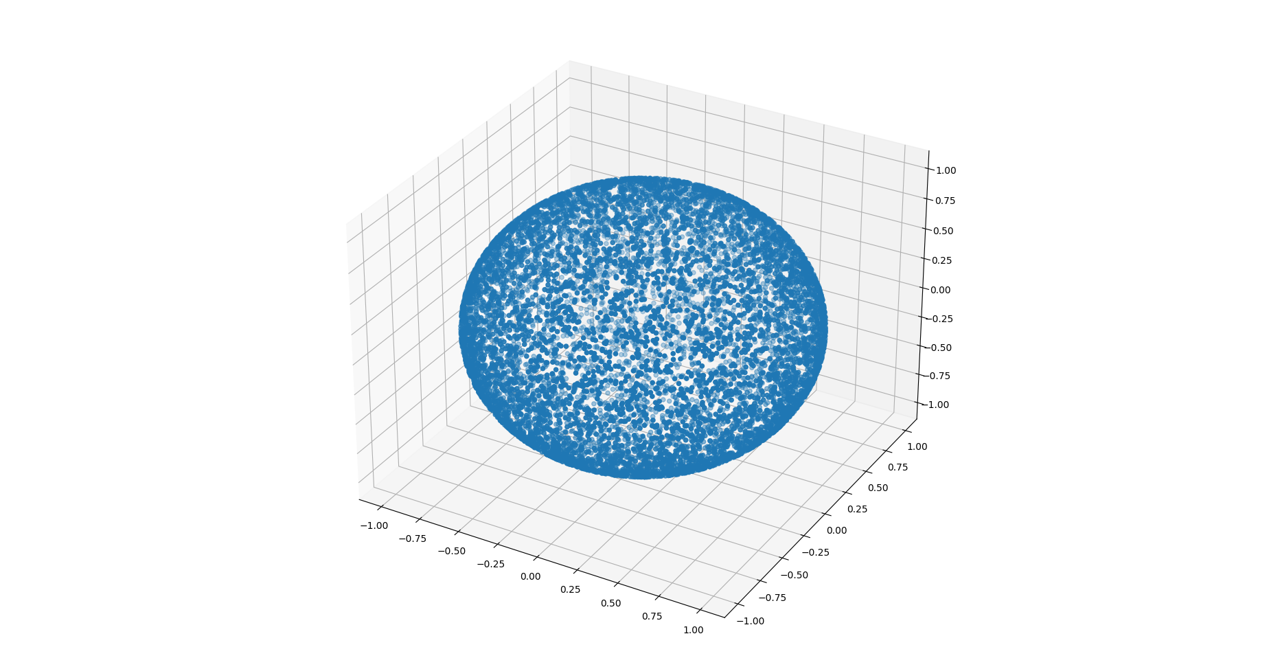
	Datasets either generated or fetched.	Authors Hind Montassif Since GUDHI 3.5.0 License MIT (LGPL v3) Requires CGAL
Datasets manual