Alpha complex user manual

Definition

	Alpha complex is a simplicial complex constructed from the finite cells of a Delaunay Triangulation. It has the same persistent homology as the Čech complex and is significantly smaller.	Author Vincent Rouvreau Since GUDHI 2.0.0 License MIT (GPL v3) Requires Eigen \(\geq\) 3.1.0 and CGAL \(\geq\) 4.11.0
Alpha complex user manual	Alpha complex reference manual

AlphaComplex is constructing a SimplexTree using Delaunay Triangulation [17] from the Computational Geometry Algorithms Library [31].

Remarks

• When an \(\alpha\)-complex is constructed with an infinite value of \(\alpha^2\), the complex is a Delaunay complex (with special filtration values). The Delaunay complex without filtration values is also available by passing default_filtration_value = True to create_simplex_tree().

• For people only interested in the topology of the Alpha complex (for instance persistence), Alpha complex is equivalent to the Čech complex and much smaller if you do not bound the radii. Čech complex can still make sense in higher dimension precisely because you can bound the radii.

• Using the default precision = 'safe' makes the construction safe. If you pass precision = 'exact' to __init__(), the filtration values are the exact ones converted to float. This can be very slow. If you pass precision = 'safe' (the default), the filtration values are only guaranteed to have a small multiplicative error compared to the exact value. A drawback, when computing persistence, is that an empty exact interval [10^12,10^12] may become a non-empty approximate interval [10^12,10^12+10^6]. Using precision = 'fast' makes the computations slightly faster, and the combinatorics are still exact, but the computation of filtration values can exceptionally be arbitrarily bad. In all cases, we still guarantee that the output is a valid filtration (faces have a filtration value no larger than their cofaces).

• For performances reasons, it is advised to use Alpha_complex with CGAL \(\geq\) 5.0.0.

• The vertices in the output simplex tree are not guaranteed to match the order of the input points. One can use get_point() to get the initial point back.

Example from points

This example builds the alpha-complex from the given points:

import gudhi
alpha_complex = gudhi.AlphaComplex(points=[[1, 1], [7, 0], [4, 6], [9, 6], [0, 14], [2, 19], [9, 17]])

simplex_tree = alpha_complex.create_simplex_tree()
result_str = 'Alpha complex is of dimension ' + repr(simplex_tree.dimension()) + ' - ' + \
    repr(simplex_tree.num_simplices()) + ' simplices - ' + \
    repr(simplex_tree.num_vertices()) + ' vertices.'
print(result_str)
fmt = '%s -> %.2f'
for filtered_value in simplex_tree.get_filtration():
    print(fmt % tuple(filtered_value))

The output is:

Alpha complex is of dimension 2 - 25 simplices - 7 vertices.
[0] -> 0.00
[1] -> 0.00
[2] -> 0.00
[3] -> 0.00
[4] -> 0.00
[5] -> 0.00
[6] -> 0.00
[2, 3] -> 6.25
[4, 5] -> 7.25
[0, 2] -> 8.50
[0, 1] -> 9.25
[1, 3] -> 10.00
[1, 2] -> 11.25
[1, 2, 3] -> 12.50
[0, 1, 2] -> 13.00
[5, 6] -> 13.25
[2, 4] -> 20.00
[4, 6] -> 22.74
[4, 5, 6] -> 22.74
[3, 6] -> 30.25
[2, 6] -> 36.50
[2, 3, 6] -> 36.50
[2, 4, 6] -> 37.24
[0, 4] -> 59.71
[0, 2, 4] -> 59.71

Algorithm

Data structure

In order to build the alpha complex, first, a Simplex tree is built from the cells of a Delaunay Triangulation. (The filtration value is set to NaN, which stands for unknown value):

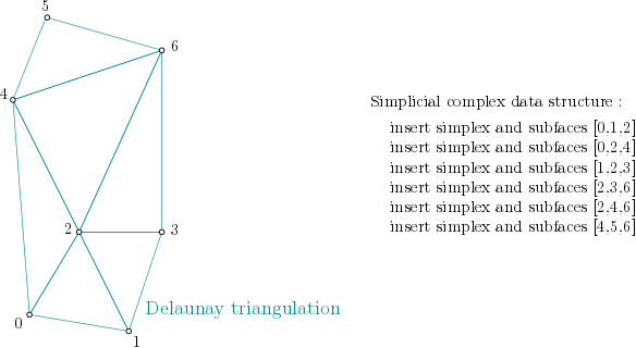
Simplex tree structure construction example

Filtration value computation algorithm

for i : dimension → 0 do
  for all σ of dimension i
    if filtration(σ) is NaN then
      filtration(σ) = α²(σ)
    end if
    for all τ face of σ do // propagate alpha filtration value
      if filtration(τ) is not NaN then
        filtration(τ) = min( filtration(τ), filtration(σ) )
      else
        if τ is not Gabriel for σ then
          filtration(τ) = filtration(σ)
        end if
      end if
    end for
  end for
end for

make_filtration_non_decreasing()
prune_above_filtration()

Dimension 2

From the example above, it means the algorithm looks into each triangle ([0,1,2], [0,2,4], [1,2,3], …), computes the filtration value of the triangle, and then propagates the filtration value as described here:

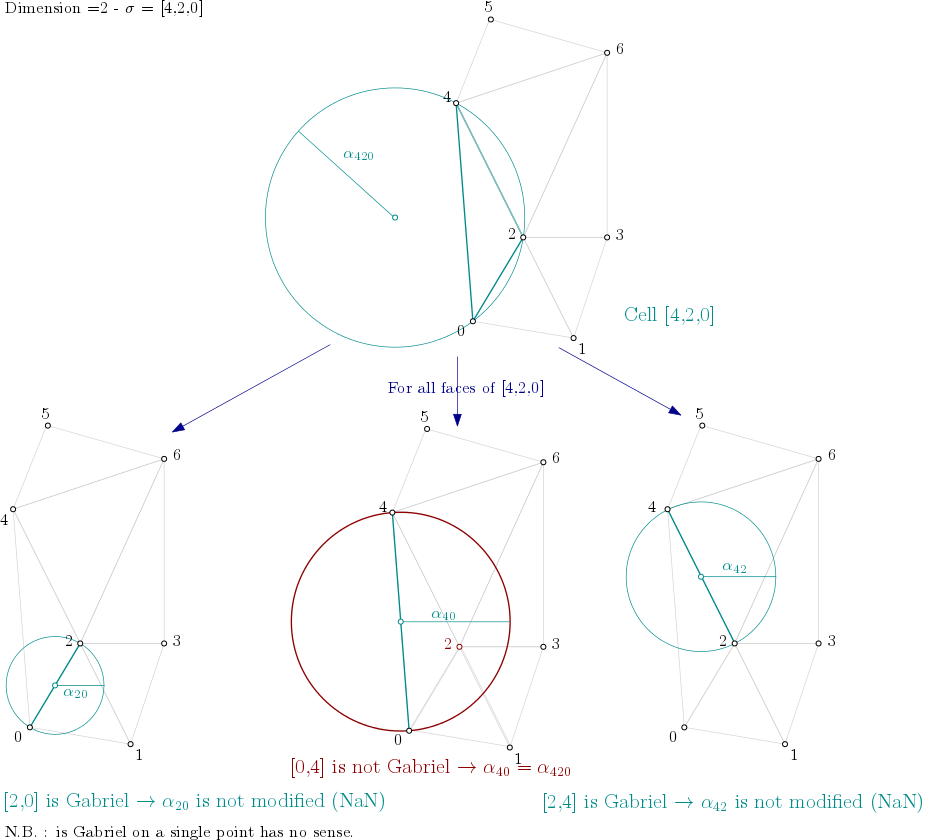
Filtration value propagation example

Dimension 1

Then, the algorithm looks into each edge ([0,1], [0,2], [1,2], …), computes the filtration value of the edge (in this case, propagation will have no effect).

Dimension 0

Finally, the algorithm looks into each vertex ([0], [1], [2], [3], [4], [5] and [6]) and sets the filtration value (0 in case of a vertex - propagation will have no effect).

Non decreasing filtration values

As the squared radii computed by CGAL are an approximation, it might happen that these \(\alpha^2\) values do not quite define a proper filtration (i.e. non-decreasing with respect to inclusion). We fix that up by calling make_filtration_non_decreasing() (cf. C++ version).

Note

This is not the case in exact version, this is the reason why it is not called in this case.

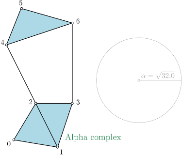
Prune above given filtration value

The simplex tree is pruned from the given maximum \(\alpha^2\) value (cf. prune_above_filtration()). Note that this does not provide any kind of speed-up, since we always first build the full filtered complex, so it is recommended not to use max_alpha_square. In the following example, a threshold of \(\alpha^2 = 32.0\) is used.

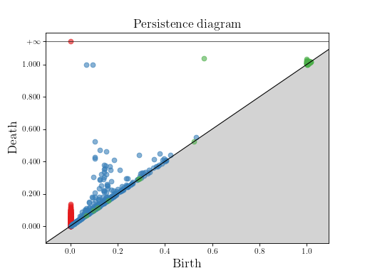
Example from OFF file

This example builds the alpha complex from 300 random points on a 2-torus.

Then, it computes the persistence diagram and displays it:

import matplotlib.pyplot as plt
import gudhi
alpha_complex = gudhi.AlphaComplex(off_file=gudhi.__root_source_dir__ + \
    '/data/points/tore3D_300.off')
simplex_tree = alpha_complex.create_simplex_tree()
result_str = 'Alpha complex is of dimension ' + repr(simplex_tree.dimension()) + ' - ' + \
    repr(simplex_tree.num_simplices()) + ' simplices - ' + \
    repr(simplex_tree.num_vertices()) + ' vertices.'
print(result_str)
diag = simplex_tree.persistence()
gudhi.plot_persistence_diagram(diag)
plt.show()