Representations manual
|
Vectorizations, distances and kernels that work on persistence diagrams, compatible with scikit-learn. |
|
This module, originally available at https://github.com/MathieuCarriere/sklearn-tda and named sklearn_tda, aims at bridging the gap between persistence diagrams and machine learning, by providing implementations of most of the vector representations for persistence diagrams in the literature, in a scikit-learn format. More specifically, it provides tools, using the scikit-learn standard interface, to compute distances and kernels on persistence diagrams, and to convert these diagrams into vectors in Euclidean space.
A diagram is represented as a numpy array of shape (n,2), as can be obtained from persistence_intervals_in_dimension() for instance. Points at infinity are represented as a numpy array of shape (n,1), storing only the birth time. The classes in this module can handle several persistence diagrams at once. In that case, the diagrams are provided as a list of numpy arrays. Note that it is not necessary for the diagrams to have the same number of points, i.e., for the corresponding arrays to have the same number of rows: all classes can handle arrays with different shapes.
Examples
Landscapes
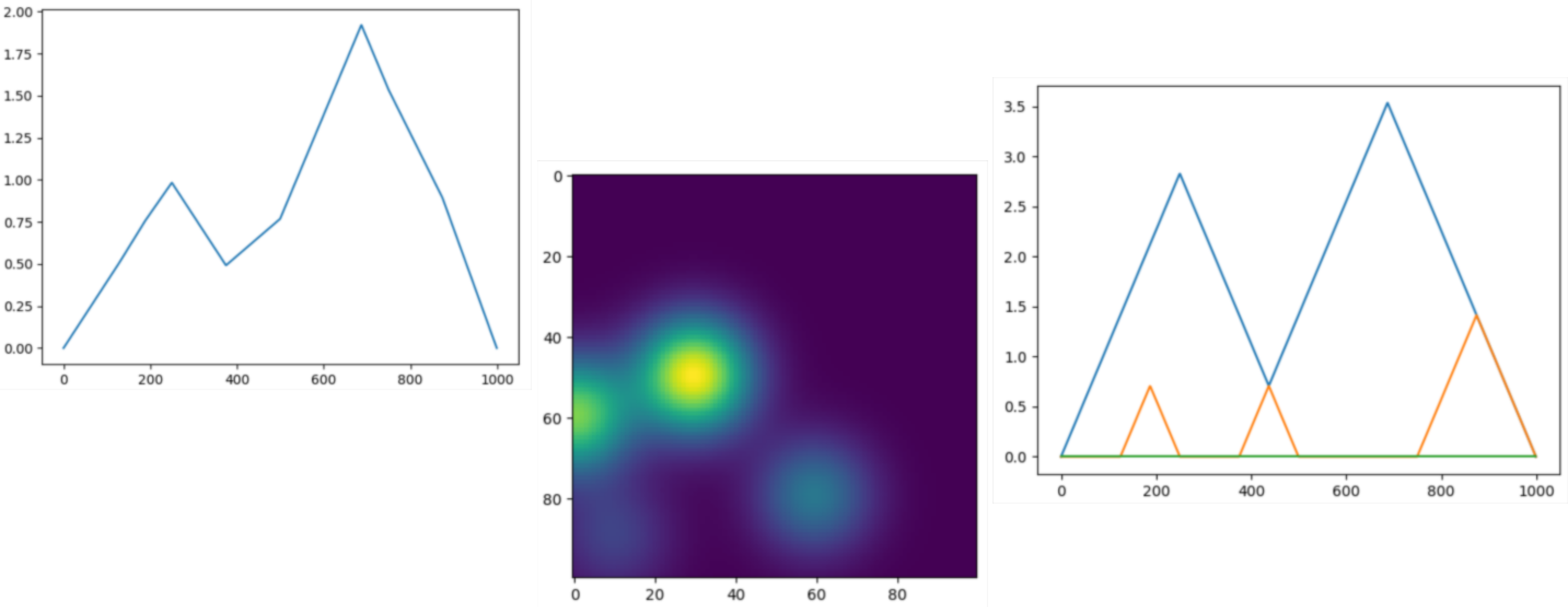
This example computes the first two Landscapes associated to a persistence diagram with four points. The landscapes are evaluated on ten samples, leading to two vectors with ten coordinates each, that are eventually concatenated in order to produce a single vector representation.
import numpy as np
from gudhi.representations import Landscape
# A single diagram with 4 points
D = np.array([[0.,4.],[1.,2.],[3.,8.],[6.,8.]])
diags = [D]
l=Landscape(num_landscapes=2,resolution=10).fit_transform(diags)
print(l)
The output is:
[[1.02851895 2.05703791 2.57129739 1.54277843 0.89995409 1.92847304
  2.95699199 3.08555686 2.05703791 1.02851895 0.         0.64282435
  0.         0.         0.51425948 0.         0.         0.
  0.77138922 1.02851895]]
Various kernels
This small example is also provided
diagram_vectorizations_distances_kernels.py
Machine Learning and Topological Data Analysis
This notebook explains how to efficiently combine machine learning and topological data analysis with the representations module.
Preprocessing
-
class
gudhi.representations.preprocessing.BirthPersistenceTransform[source]¶ Bases:
sklearn.base.BaseEstimator,sklearn.base.TransformerMixinThis is a class for the affine transformation (x,y) -> (x,y-x) to be applied on persistence diagrams.
-
__call__(diag)[source]¶ Apply BirthPersistenceTransform on a single persistence diagram and outputs the result.
- Parameters
diag¶ (n x 2 numpy array) – input persistence diagram.
- Returns
transformed persistence diagram.
- Return type
n x 2 numpy array
-
-
class
gudhi.representations.preprocessing.Clamping(minimum=-inf, maximum=inf)[source]¶ Bases:
sklearn.base.BaseEstimator,sklearn.base.TransformerMixinThis is a class for clamping values. It can be used as a parameter for the DiagramScaler class, for instance if you want to clamp abscissae or ordinates of persistence diagrams.
-
__init__(minimum=-inf, maximum=inf)[source]¶ Constructor for the Clamping class.
- Parameters
limit¶ (double) – clamping value (default np.inf).
-
-
class
gudhi.representations.preprocessing.DiagramScaler(use=False, scalers=[])[source]¶ Bases:
sklearn.base.BaseEstimator,sklearn.base.TransformerMixinThis is a class for preprocessing persistence diagrams with a given list of scalers, such as those included in scikit-learn.
-
__call__(diag)[source]¶ Apply DiagramScaler on a single persistence diagram and outputs the result.
- Parameters
diag¶ (n x 2 numpy array) – input persistence diagram.
- Returns
transformed persistence diagram.
- Return type
n x 2 numpy array
-
__init__(use=False, scalers=[])[source]¶ Constructor for the DiagramScaler class.
- Parameters
use¶ (bool) – whether to use the class or not (default False).
scalers¶ (list of classes) – list of scalers to be fit on the persistence diagrams (default []). Each element of the list is a tuple with two elements: the first one is a list of coordinates, and the second one is a scaler (i.e. a class with fit() and transform() methods) that is going to be applied to these coordinates. Common scalers can be found in the scikit-learn library (such as MinMaxScaler for instance).
-
fit(X, y=None)[source]¶ Fit the DiagramScaler class on a list of persistence diagrams: persistence diagrams are concatenated in a big numpy array, and scalers are fit (by calling their fit() method) on their corresponding coordinates in this big array.
-
transform(X)[source]¶ Apply the DiagramScaler function on the persistence diagrams. The fitted scalers are applied (by calling their transform() method) to their corresponding coordinates in each persistence diagram individually.
- Parameters
X¶ (list of n x 2 or n x 1 numpy arrays) – input persistence diagrams.
- Returns
transformed persistence diagrams.
- Return type
list of n x 2 or n x 1 numpy arrays
-
-
class
gudhi.representations.preprocessing.DiagramSelector(use=False, limit=inf, point_type='finite')[source]¶ Bases:
sklearn.base.BaseEstimator,sklearn.base.TransformerMixinThis is a class for extracting finite or essential points in persistence diagrams.
-
__call__(diag)[source]¶ Apply DiagramSelector on a single persistence diagram and outputs the result.
- Parameters
diag¶ (n x 2 numpy array) – input persistence diagram.
- Returns
extracted persistence diagram.
- Return type
n x 2 numpy array
-
__init__(use=False, limit=inf, point_type='finite')[source]¶ Constructor for the DiagramSelector class.
-
-
class
gudhi.representations.preprocessing.Padding(use=False)[source]¶ Bases:
sklearn.base.BaseEstimator,sklearn.base.TransformerMixinThis is a class for padding a list of persistence diagrams with dummy points, so that all persistence diagrams end up with the same number of points.
-
__call__(diag)[source]¶ Apply Padding on a single persistence diagram and outputs the result.
- Parameters
diag¶ (n x 2 numpy array) – input persistence diagram.
- Returns
padded persistence diagram.
- Return type
n x 2 numpy array
-
__init__(use=False)[source]¶ Constructor for the Padding class.
- Parameters
use¶ (bool) – whether to use the class or not (default False).
-
fit(X, y=None)[source]¶ Fit the Padding class on a list of persistence diagrams (this function actually does nothing but is useful when Padding is included in a scikit-learn Pipeline).
-
transform(X)[source]¶ Add dummy points to each persistence diagram so that they all have the same cardinality. All points are given an additional coordinate indicating if the point was added after padding (0) or already present before (1).
- Parameters
X¶ (list of n x 2 or n x 1 numpy arrays) – input persistence diagrams.
- Returns
padded persistence diagrams.
- Return type
list of n x 3 or n x 2 numpy arrays
-
-
class
gudhi.representations.preprocessing.ProminentPoints(use=False, num_pts=10, threshold=-1, location='upper')[source]¶ Bases:
sklearn.base.BaseEstimator,sklearn.base.TransformerMixinThis is a class for removing points that are close or far from the diagonal in persistence diagrams. If persistence diagrams are n x 2 numpy arrays (i.e. persistence diagrams with ordinary features), points are ordered and thresholded by distance-to-diagonal. If persistence diagrams are n x 1 numpy arrays (i.e. persistence diagrams with essential features), points are not ordered and thresholded by first coordinate.
-
__call__(diag)[source]¶ Apply ProminentPoints on a single persistence diagram and outputs the result.
- Parameters
diag¶ (n x 2 numpy array) – input persistence diagram.
- Returns
thresholded persistence diagram.
- Return type
n x 2 numpy array
-
__init__(use=False, num_pts=10, threshold=-1, location='upper')[source]¶ Constructor for the ProminentPoints class.
- Parameters
use¶ (bool) – whether to use the class or not (default False).
location¶ (string) – either “upper” or “lower” (default “upper”). Whether to keep the points that are far away (“upper”) or close (“lower”) to the diagonal.
num_pts¶ (int) – cardinality threshold (default 10). If location == “upper”, keep the top num_pts points that are the farthest away from the diagonal. If location == “lower”, keep the top num_pts points that are the closest to the diagonal.
threshold¶ (double) – distance-to-diagonal threshold (default -1). If location == “upper”, keep the points that are at least at a distance threshold from the diagonal. If location == “lower”, keep the points that are at most at a distance threshold from the diagonal.
-
fit(X, y=None)[source]¶ Fit the ProminentPoints class on a list of persistence diagrams (this function actually does nothing but is useful when ProminentPoints is included in a scikit-learn Pipeline).
-
transform(X)[source]¶ If location == “upper”, first select the top num_pts points that are the farthest away from the diagonal, then select and return from these points the ones that are at least at distance threshold from the diagonal for each persistence diagram individually. If location == “lower”, first select the top num_pts points that are the closest to the diagonal, then select and return from these points the ones that are at most at distance threshold from the diagonal for each persistence diagram individually.
- Parameters
X¶ (list of n x 2 or n x 1 numpy arrays) – input persistence diagrams.
- Returns
thresholded persistence diagrams.
- Return type
list of n x 2 or n x 1 numpy arrays
-
Vector methods
-
class
gudhi.representations.vector_methods.Atol(quantiser, weighting_method='cloud', contrast='gaussian')[source]¶ Bases:
sklearn.base.BaseEstimator,sklearn.base.TransformerMixinThis class allows to vectorise measures (e.g. point clouds, persistence diagrams, etc) after a quantisation step.
ATOL paper: [26]
Example
>>> from sklearn.cluster import KMeans
>>> from gudhi.representations.vector_methods import Atol
>>> import numpy as np
>>> a = np.array([[1, 2, 4], [1, 4, 0], [1, 0, 4]])
>>> b = np.array([[4, 2, 0], [4, 4, 0], [4, 0, 2]])
>>> c = np.array([[3, 2, -1], [1, 2, -1]])
>>> atol_vectoriser = Atol(quantiser=KMeans(n_clusters=2, random_state=202006))
>>> atol_vectoriser.fit(X=[a, b, c]).centers
array([[ 2.        ,  0.66666667,  3.33333333],
       [ 2.6       ,  2.8       , -0.4       ]])
>>> atol_vectoriser(a)
array([1.18168665, 0.42375966])
>>> atol_vectoriser(c)
array([0.02062512, 1.25157463])
>>> atol_vectoriser.transform(X=[a, b, c])
array([[1.18168665, 0.42375966],
       [0.29861028, 1.06330156],
       [0.02062512, 1.25157463]])
-
__call__(measure, sample_weight=None)[source]¶ Apply measure vectorisation on a single measure.
- Parameters
measure¶ (n x d numpy array) – input measure in R^d.
- Returns
numpy array in R^self.quantiser.n_clusters.
-
__init__(quantiser, weighting_method='cloud', contrast='gaussian')[source]¶ Constructor for the Atol measure vectorisation class.
- Parameters
quantiser¶ (Object) – Object with fit (sklearn API consistent) and cluster_centers and n_clusters attributes, e.g. sklearn.cluster.KMeans. It will be fitted when the Atol object function fit is called.
weighting_method¶ (string) – constant generic function for weighting the measure points choose from {“cloud”, “iidproba”} (default: constant function, i.e. the measure is seen as a point cloud by default). This will have no impact if weights are provided along with measures all the way: fit and transform.
contrast¶ (string) – constant function for evaluating proximity of a measure with respect to centers choose from {“gaussian”, “laplacian”, “indicator”} (default: gaussian contrast function, see page 3 in the ATOL paper).
-
fit(X, y=None, sample_weight=None)[source]¶ Calibration step: fit centers to the sample measures and derive inertias between centers.
- Parameters
X¶ (list N x d numpy arrays) – input measures in R^d from which to learn center locations and inertias (measures can have different N).
y¶ – Ignored, present for API consistency by convention.
sample_weight¶ (list of numpy arrays) – weights for each measure point in X, optional. If None, the object’s weighting_method will be used.
- Returns
self
-
-
class
gudhi.representations.vector_methods.BettiCurve(resolution=100, sample_range=[nan, nan])[source]¶ Bases:
sklearn.base.BaseEstimator,sklearn.base.TransformerMixinThis is a class for computing Betti curves from a list of persistence diagrams. A Betti curve is a 1D piecewise-constant function obtained from the rank function. It is sampled evenly on a given range and the vector of samples is returned. See https://www.researchgate.net/publication/316604237_Time_Series_Classification_via_Topological_Data_Analysis for more details.
-
__call__(diag)[source]¶ Apply BettiCurve on a single persistence diagram and outputs the result.
- Parameters
diag¶ (n x 2 numpy array) – input persistence diagram.
- Returns
output Betti curve.
- Return type
numpy array with shape (resolution)
-
__init__(resolution=100, sample_range=[nan, nan])[source]¶ Constructor for the BettiCurve class.
- Parameters
resolution¶ (int) – number of sample for the piecewise-constant function (default 100).
sample_range¶ ([double, double]) – minimum and maximum of the piecewise-constant function domain, of the form [x_min, x_max] (default [numpy.nan, numpy.nan]). It is the interval on which samples will be drawn evenly. If one of the values is numpy.nan, it can be computed from the persistence diagrams with the fit() method.
-
-
class
gudhi.representations.vector_methods.ComplexPolynomial(polynomial_type='R', threshold=10)[source]¶ Bases:
sklearn.base.BaseEstimator,sklearn.base.TransformerMixinThis is a class for computing complex polynomials from a list of persistence diagrams. The persistence diagram points are seen as the roots of some complex polynomial, whose coefficients are returned in a complex vector. See https://link.springer.com/chapter/10.1007%2F978-3-319-23231-7_27 for more details.
-
__call__(diag)[source]¶ Apply ComplexPolynomial on a single persistence diagram and outputs the result.
- Parameters
diag¶ (n x 2 numpy array) – input persistence diagram.
- Returns
output complex vector of coefficients.
- Return type
numpy array with shape (threshold)
-
__init__(polynomial_type='R', threshold=10)[source]¶ Constructor for the ComplexPolynomial class.
- Parameters
polynomial_type¶ (char) – either “R”, “S” or “T” (default “R”). Type of complex polynomial that is going to be computed (explained in https://link.springer.com/chapter/10.1007%2F978-3-319-23231-7_27).
threshold¶ (int) – number of coefficients (default 10). This is the dimension of the complex vector of coefficients, i.e. the number of coefficients corresponding to the largest degree terms of the polynomial. If -1, this threshold is computed from the list of persistence diagrams by considering the one with the largest number of points and using the dimension of its corresponding complex vector of coefficients as threshold.
-
fit(X, y=None)[source]¶ Fit the ComplexPolynomial class on a list of persistence diagrams (this function actually does nothing but is useful when ComplexPolynomial is included in a scikit-learn Pipeline).
-
transform(X)[source]¶ Compute the complex vector of coefficients for each persistence diagram individually and concatenate the results.
- Parameters
X¶ (list of n x 2 numpy arrays) – input persistence diagrams.
- Returns
output complex vectors of coefficients.
- Return type
numpy array with shape (number of diagrams) x (threshold)
-
-
class
gudhi.representations.vector_methods.Entropy(mode='scalar', normalized=True, resolution=100, sample_range=[nan, nan])[source]¶ Bases:
sklearn.base.BaseEstimator,sklearn.base.TransformerMixinThis is a class for computing persistence entropy. Persistence entropy is a statistic for persistence diagrams inspired from Shannon entropy. This statistic can also be used to compute a feature vector, called the entropy summary function. See https://arxiv.org/pdf/1803.08304.pdf for more details. Note that a previous implementation was contributed by Manuel Soriano-Trigueros.
-
__call__(diag)[source]¶ Apply Entropy on a single persistence diagram and outputs the result.
- Parameters
diag¶ (n x 2 numpy array) – input persistence diagram.
- Returns
output entropy.
- Return type
numpy array with shape (1 if mode = “scalar” else resolution)
-
__init__(mode='scalar', normalized=True, resolution=100, sample_range=[nan, nan])[source]¶ Constructor for the Entropy class.
- Parameters
mode¶ (string) – what entropy to compute: either “scalar” for computing the entropy statistics, or “vector” for computing the entropy summary functions (default “scalar”).
normalized¶ (bool) – whether to normalize the entropy summary function (default True). Used only if mode = “vector”.
resolution¶ (int) – number of sample for the entropy summary function (default 100). Used only if mode = “vector”.
sample_range¶ ([double, double]) – minimum and maximum of the entropy summary function domain, of the form [x_min, x_max] (default [numpy.nan, numpy.nan]). It is the interval on which samples will be drawn evenly. If one of the values is numpy.nan, it can be computed from the persistence diagrams with the fit() method. Used only if mode = “vector”.
-
transform(X)[source]¶ Compute the entropy for each persistence diagram individually and concatenate the results.
- Parameters
X¶ (list of n x 2 numpy arrays) – input persistence diagrams.
- Returns
output entropy.
- Return type
numpy array with shape (number of diagrams) x (1 if mode = “scalar” else resolution)
-
-
class
gudhi.representations.vector_methods.Landscape(num_landscapes=5, resolution=100, sample_range=[nan, nan])[source]¶ Bases:
sklearn.base.BaseEstimator,sklearn.base.TransformerMixinThis is a class for computing persistence landscapes from a list of persistence diagrams. A persistence landscape is a collection of 1D piecewise-linear functions computed from the rank function associated to the persistence diagram. These piecewise-linear functions are then sampled evenly on a given range and the corresponding vectors of samples are concatenated and returned. See http://jmlr.org/papers/v16/bubenik15a.html for more details.
-
__call__(diag)[source]¶ Apply Landscape on a single persistence diagram and outputs the result.
- Parameters
diag¶ (n x 2 numpy array) – input persistence diagram.
- Returns
output persistence landscape.
- Return type
numpy array with shape (number of samples = num_landscapes x resolution)
-
__init__(num_landscapes=5, resolution=100, sample_range=[nan, nan])[source]¶ Constructor for the Landscape class.
- Parameters
num_landscapes¶ (int) – number of piecewise-linear functions to output (default 5).
resolution¶ (int) – number of sample for all piecewise-linear functions (default 100).
sample_range¶ ([double, double]) – minimum and maximum of all piecewise-linear function domains, of the form [x_min, x_max] (default [numpy.nan, numpy.nan]). It is the interval on which samples will be drawn evenly. If one of the values is numpy.nan, it can be computed from the persistence diagrams with the fit() method.
-
fit(X, y=None)[source]¶ Fit the Landscape class on a list of persistence diagrams: if any of the values in sample_range is numpy.nan, replace it with the corresponding value computed on the given list of persistence diagrams.
-
transform(X)[source]¶ Compute the persistence landscape for each persistence diagram individually and concatenate the results.
- Parameters
X¶ (list of n x 2 numpy arrays) – input persistence diagrams.
- Returns
output persistence landscapes.
- Return type
numpy array with shape (number of diagrams) x (number of samples = num_landscapes x resolution)
-
-
class
gudhi.representations.vector_methods.PersistenceImage(bandwidth=1.0, weight=<function PersistenceImage.<lambda>>, resolution=[20, 20], im_range=[nan, nan, nan, nan])[source]¶ Bases:
sklearn.base.BaseEstimator,sklearn.base.TransformerMixinThis is a class for computing persistence images from a list of persistence diagrams. A persistence image is a 2D function computed from a persistence diagram by convolving the diagram points with a weighted Gaussian kernel. The plane is then discretized into an image with pixels, which is flattened and returned as a vector. See http://jmlr.org/papers/v18/16-337.html for more details.
-
__call__(diag)[source]¶ Apply PersistenceImage on a single persistence diagram and outputs the result.
- Parameters
diag¶ (n x 2 numpy array) – input persistence diagram.
- Returns
numpy array with shape (number of pixels = resolution[0] x resolution[1]):: output persistence image.
-
__init__(bandwidth=1.0, weight=<function PersistenceImage.<lambda>>, resolution=[20, 20], im_range=[nan, nan, nan, nan])[source]¶ Constructor for the PersistenceImage class.
- Parameters
bandwidth¶ (double) – bandwidth of the Gaussian kernel (default 1.).
weight¶ (function) – weight function for the persistence diagram points (default constant function, ie lambda x: 1). This function must be defined on 2D points, ie lists or numpy arrays of the form [p_x,p_y].
resolution¶ ([int,int]) – size (in pixels) of the persistence image (default [20,20]).
im_range¶ ([double,double,double,double]) – minimum and maximum of each axis of the persistence image, of the form [x_min, x_max, y_min, y_max] (default [numpy.nan, numpy.nan, numpy.nan, numpyp.nan]). If one of the values is numpy.nan, it can be computed from the persistence diagrams with the fit() method.
-
fit(X, y=None)[source]¶ Fit the PersistenceImage class on a list of persistence diagrams: if any of the values in im_range is numpy.nan, replace it with the corresponding value computed on the given list of persistence diagrams.
-
transform(X)[source]¶ Compute the persistence image for each persistence diagram individually and store the results in a single numpy array.
- Parameters
X¶ (list of n x 2 numpy arrays) – input persistence diagrams.
- Returns
output persistence images.
- Return type
numpy array with shape (number of diagrams) x (number of pixels = resolution[0] x resolution[1])
-
-
class
gudhi.representations.vector_methods.Silhouette(weight=<function Silhouette.<lambda>>, resolution=100, sample_range=[nan, nan])[source]¶ Bases:
sklearn.base.BaseEstimator,sklearn.base.TransformerMixinThis is a class for computing persistence silhouettes from a list of persistence diagrams. A persistence silhouette is computed by taking a weighted average of the collection of 1D piecewise-linear functions given by the persistence landscapes, and then by evenly sampling this average on a given range. Finally, the corresponding vector of samples is returned. See https://arxiv.org/abs/1312.0308 for more details.
-
__call__(diag)[source]¶ Apply Silhouette on a single persistence diagram and outputs the result.
- Parameters
diag¶ (n x 2 numpy array) – input persistence diagram.
- Returns
output persistence silhouette.
- Return type
numpy array with shape (resolution)
-
__init__(weight=<function Silhouette.<lambda>>, resolution=100, sample_range=[nan, nan])[source]¶ Constructor for the Silhouette class.
- Parameters
weight¶ (function) – weight function for the persistence diagram points (default constant function, ie lambda x: 1). This function must be defined on 2D points, ie on lists or numpy arrays of the form [p_x,p_y].
resolution¶ (int) – number of samples for the weighted average (default 100).
sample_range¶ ([double, double]) – minimum and maximum for the weighted average domain, of the form [x_min, x_max] (default [numpy.nan, numpy.nan]). It is the interval on which samples will be drawn evenly. If one of the values is numpy.nan, it can be computed from the persistence diagrams with the fit() method.
-
fit(X, y=None)[source]¶ Fit the Silhouette class on a list of persistence diagrams: if any of the values in sample_range is numpy.nan, replace it with the corresponding value computed on the given list of persistence diagrams.
-
transform(X)[source]¶ Compute the persistence silhouette for each persistence diagram individually and concatenate the results.
- Parameters
X¶ (list of n x 2 numpy arrays) – input persistence diagrams.
- Returns
output persistence silhouettes.
- Return type
numpy array with shape (number of diagrams) x (resolution)
-
-
class
gudhi.representations.vector_methods.TopologicalVector(threshold=10)[source]¶ Bases:
sklearn.base.BaseEstimator,sklearn.base.TransformerMixinThis is a class for computing topological vectors from a list of persistence diagrams. The topological vector associated to a persistence diagram is the sorted vector of a slight modification of the pairwise distances between the persistence diagram points. See https://diglib.eg.org/handle/10.1111/cgf12692 for more details.
-
__call__(diag)[source]¶ Apply TopologicalVector on a single persistence diagram and outputs the result.
- Parameters
diag¶ (n x 2 numpy array) – input persistence diagram.
- Returns
output topological vector.
- Return type
numpy array with shape (threshold)
-
__init__(threshold=10)[source]¶ Constructor for the TopologicalVector class.
- Parameters
threshold¶ (int) – number of distances to keep (default 10). This is the dimension of the topological vector. If -1, this threshold is computed from the list of persistence diagrams by considering the one with the largest number of points and using the dimension of its corresponding topological vector as threshold.
-
fit(X, y=None)[source]¶ Fit the TopologicalVector class on a list of persistence diagrams (this function actually does nothing but is useful when TopologicalVector is included in a scikit-learn Pipeline).
-
transform(X)[source]¶ Compute the topological vector for each persistence diagram individually and concatenate the results.
- Parameters
X¶ (list of n x 2 numpy arrays) – input persistence diagrams.
- Returns
output topological vectors.
- Return type
numpy array with shape (number of diagrams) x (threshold)
-
Kernel methods
-
class
gudhi.representations.kernel_methods.PersistenceFisherKernel(bandwidth_fisher=1.0, bandwidth=1.0, kernel_approx=None, n_jobs=None)[source]¶ Bases:
sklearn.base.BaseEstimator,sklearn.base.TransformerMixinThis is a class for computing the persistence Fisher kernel matrix from a list of persistence diagrams. The persistence Fisher kernel is computed by exponentiating the corresponding persistence Fisher distance with a Gaussian kernel. See papers.nips.cc/paper/8205-persistence-fisher-kernel-a-riemannian-manifold-kernel-for-persistence-diagrams for more details.
-
__call__(diag1, diag2)[source]¶ Apply PersistenceFisherKernel on a single pair of persistence diagrams and outputs the result.
-
__init__(bandwidth_fisher=1.0, bandwidth=1.0, kernel_approx=None, n_jobs=None)[source]¶ Constructor for the PersistenceFisherKernel class.
- Parameters
bandwidth¶ (double) – bandwidth of the Gaussian kernel applied to the persistence Fisher distance (default 1.).
bandwidth_fisher¶ (double) – bandwidth of the Gaussian kernel used to turn persistence diagrams into probability distributions by PersistenceFisherDistance class (default 1.).
kernel_approx¶ (class) – kernel approximation class used to speed up computation (default None). Common kernel approximations classes can be found in the scikit-learn library (such as RBFSampler for instance).
n_jobs¶ (int) – number of jobs to use for the computation. See
pairwise_persistence_diagram_kernels()for details.
-
fit(X, y=None)[source]¶ Fit the PersistenceFisherKernel class on a list of persistence diagrams: an instance of the PersistenceFisherDistance class is fitted on the diagrams and then stored.
-
transform(X)[source]¶ Compute all persistence Fisher kernel values between the persistence diagrams that were stored after calling the fit() method, and a given list of (possibly different) persistence diagrams.
- Parameters
X¶ (list of n x 2 numpy arrays) – input persistence diagrams.
- Returns
matrix of pairwise persistence Fisher kernel values.
- Return type
numpy array of shape (number of diagrams in diagrams) x (number of diagrams in X)
-
-
class
gudhi.representations.kernel_methods.PersistenceScaleSpaceKernel(bandwidth=1.0, kernel_approx=None, n_jobs=None)[source]¶ Bases:
sklearn.base.BaseEstimator,sklearn.base.TransformerMixinThis is a class for computing the persistence scale space kernel matrix from a list of persistence diagrams. The persistence scale space kernel is computed by adding the symmetric to the diagonal of each point in each persistence diagram, with negative weight, and then convolving the points with a Gaussian kernel. See https://www.cv-foundation.org/openaccess/content_cvpr_2015/papers/Reininghaus_A_Stable_Multi-Scale_2015_CVPR_paper.pdf for more details.
-
__call__(diag1, diag2)[source]¶ Apply PersistenceScaleSpaceKernel on a single pair of persistence diagrams and outputs the result.
-
__init__(bandwidth=1.0, kernel_approx=None, n_jobs=None)[source]¶ Constructor for the PersistenceScaleSpaceKernel class.
- Parameters
bandwidth¶ (double) – bandwidth of the Gaussian kernel with which persistence diagrams will be convolved (default 1.)
kernel_approx¶ (class) – kernel approximation class used to speed up computation (default None). Common kernel approximations classes can be found in the scikit-learn library (such as RBFSampler for instance).
n_jobs¶ (int) – number of jobs to use for the computation. See
pairwise_persistence_diagram_kernels()for details.
-
fit(X, y=None)[source]¶ Fit the PersistenceScaleSpaceKernel class on a list of persistence diagrams: symmetric to the diagonal of all points are computed and an instance of the PersistenceWeightedGaussianKernel class is fitted on the diagrams and then stored.
-
transform(X)[source]¶ Compute all persistence scale space kernel values between the persistence diagrams that were stored after calling the fit() method, and a given list of (possibly different) persistence diagrams.
- Parameters
X¶ (list of n x 2 numpy arrays) – input persistence diagrams.
- Returns
matrix of pairwise persistence scale space kernel values.
- Return type
numpy array of shape (number of diagrams in diagrams) x (number of diagrams in X)
-
-
class
gudhi.representations.kernel_methods.PersistenceWeightedGaussianKernel(bandwidth=1.0, weight=<function PersistenceWeightedGaussianKernel.<lambda>>, kernel_approx=None, n_jobs=None)[source]¶ Bases:
sklearn.base.BaseEstimator,sklearn.base.TransformerMixinThis is a class for computing the persistence weighted Gaussian kernel matrix from a list of persistence diagrams. The persistence weighted Gaussian kernel is computed by convolving the persistence diagram points with weighted Gaussian kernels. See http://proceedings.mlr.press/v48/kusano16.html for more details.
-
__call__(diag1, diag2)[source]¶ Apply PersistenceWeightedGaussianKernel on a single pair of persistence diagrams and outputs the result.
-
__init__(bandwidth=1.0, weight=<function PersistenceWeightedGaussianKernel.<lambda>>, kernel_approx=None, n_jobs=None)[source]¶ Constructor for the PersistenceWeightedGaussianKernel class.
- Parameters
bandwidth¶ (double) – bandwidth of the Gaussian kernel with which persistence diagrams will be convolved (default 1.)
weight¶ (function) – weight function for the persistence diagram points (default constant function, ie lambda x: 1). This function must be defined on 2D points, ie lists or numpy arrays of the form [p_x,p_y].
kernel_approx¶ (class) – kernel approximation class used to speed up computation (default None). Common kernel approximations classes can be found in the scikit-learn library (such as RBFSampler for instance).
n_jobs¶ (int) – number of jobs to use for the computation. See
pairwise_persistence_diagram_kernels()for details.
-
fit(X, y=None)[source]¶ Fit the PersistenceWeightedGaussianKernel class on a list of persistence diagrams: persistence diagrams are stored in a numpy array called diagrams and the kernel approximation class (if not None) is applied on them.
-
transform(X)[source]¶ Compute all persistence weighted Gaussian kernel values between the persistence diagrams that were stored after calling the fit() method, and a given list of (possibly different) persistence diagrams.
- Parameters
X¶ (list of n x 2 numpy arrays) – input persistence diagrams.
- Returns
matrix of pairwise persistence weighted Gaussian kernel values.
- Return type
numpy array of shape (number of diagrams in diagrams) x (number of diagrams in X)
-
-
class
gudhi.representations.kernel_methods.SlicedWassersteinKernel(num_directions=10, bandwidth=1.0, n_jobs=None)[source]¶ Bases:
sklearn.base.BaseEstimator,sklearn.base.TransformerMixinThis is a class for computing the sliced Wasserstein kernel matrix from a list of persistence diagrams. The sliced Wasserstein kernel is computed by exponentiating the corresponding sliced Wasserstein distance with a Gaussian kernel. See http://proceedings.mlr.press/v70/carriere17a.html for more details.
-
__call__(diag1, diag2)[source]¶ Apply SlicedWassersteinKernel on a single pair of persistence diagrams and outputs the result.
-
__init__(num_directions=10, bandwidth=1.0, n_jobs=None)[source]¶ Constructor for the SlicedWassersteinKernel class.
- Parameters
bandwidth¶ (double) – bandwidth of the Gaussian kernel applied to the sliced Wasserstein distance (default 1.).
num_directions¶ (int) – number of lines evenly sampled from [-pi/2,pi/2] in order to approximate and speed up the kernel computation (default 10).
n_jobs¶ (int) – number of jobs to use for the computation. See
pairwise_persistence_diagram_kernels()for details.
-
fit(X, y=None)[source]¶ Fit the SlicedWassersteinKernel class on a list of persistence diagrams: an instance of the SlicedWassersteinDistance class is fitted on the diagrams and then stored.
-
transform(X)[source]¶ Compute all sliced Wasserstein kernel values between the persistence diagrams that were stored after calling the fit() method, and a given list of (possibly different) persistence diagrams.
- Parameters
X¶ (list of n x 2 numpy arrays) – input persistence diagrams.
- Returns
matrix of pairwise sliced Wasserstein kernel values.
- Return type
numpy array of shape (number of diagrams in diagrams) x (number of diagrams in X)
-
-
gudhi.representations.kernel_methods.pairwise_persistence_diagram_kernels(X, Y=None, kernel='sliced_wasserstein', n_jobs=None, **kwargs)[source]¶ This function computes the kernel matrix between two lists of persistence diagrams given as numpy arrays of shape (nx2).
- Parameters
X¶ (list of n numpy arrays of shape (numx2)) – first list of persistence diagrams.
Y¶ (list of m numpy arrays of shape (numx2)) – second list of persistence diagrams (optional). If None, pairwise kernel values are computed from the first list only.
kernel¶ – kernel to use. It can be either a string (“sliced_wasserstein”, “persistence_scale_space”, “persistence_weighted_gaussian”, “persistence_fisher”) or a function taking two numpy arrays of shape (nx2) and (mx2) as inputs. If it is a function, make sure that it is symmetric.
n_jobs¶ (int) – number of jobs to use for the computation. This uses joblib.Parallel(prefer=”threads”), so kernels that do not release the GIL may not scale unless run inside a joblib.parallel_backend block.
**kwargs¶ – optional keyword parameters. Any further parameters are passed directly to the kernel function. See the docs of the various kernel classes in this module.
- Returns
kernel matrix.
- Return type
numpy array of shape (nxm)
Metrics
-
class
gudhi.representations.metrics.BottleneckDistance(epsilon=None, n_jobs=None)[source]¶ Bases:
sklearn.base.BaseEstimator,sklearn.base.TransformerMixinThis is a class for computing the bottleneck distance matrix from a list of persistence diagrams.
- Requires
CGAL \(\geq\) 4.11.0
-
__call__(diag1, diag2)[source]¶ Apply BottleneckDistance on a single pair of persistence diagrams and outputs the result.
-
__init__(epsilon=None, n_jobs=None)[source]¶ Constructor for the BottleneckDistance class.
- Parameters
epsilon¶ (double) – absolute (additive) error tolerated on the distance (default is the smallest positive float), see
gudhi.bottleneck_distance().n_jobs¶ (int) – number of jobs to use for the computation. See
pairwise_persistence_diagram_distances()for details.
-
fit(X, y=None)[source]¶ Fit the BottleneckDistance class on a list of persistence diagrams: persistence diagrams are stored in a numpy array called diagrams.
-
transform(X)[source]¶ Compute all bottleneck distances between the persistence diagrams that were stored after calling the fit() method, and a given list of (possibly different) persistence diagrams.
- Parameters
X¶ (list of n x 2 numpy arrays) – input persistence diagrams.
- Returns
matrix of pairwise bottleneck distances.
- Return type
numpy array of shape (number of diagrams in diagrams) x (number of diagrams in X)
-
class
gudhi.representations.metrics.PersistenceFisherDistance(bandwidth=1.0, kernel_approx=None, n_jobs=None)[source]¶ Bases:
sklearn.base.BaseEstimator,sklearn.base.TransformerMixinThis is a class for computing the persistence Fisher distance matrix from a list of persistence diagrams. The persistence Fisher distance is obtained by computing the original Fisher distance between the probability distributions associated to the persistence diagrams given by convolving them with a Gaussian kernel. See http://papers.nips.cc/paper/8205-persistence-fisher-kernel-a-riemannian-manifold-kernel-for-persistence-diagrams for more details.
-
__call__(diag1, diag2)[source]¶ Apply PersistenceFisherDistance on a single pair of persistence diagrams and outputs the result.
-
__init__(bandwidth=1.0, kernel_approx=None, n_jobs=None)[source]¶ Constructor for the PersistenceFisherDistance class.
- Parameters
bandwidth¶ (double) – bandwidth of the Gaussian kernel used to turn persistence diagrams into probability distributions (default 1.).
kernel_approx¶ (class) – kernel approximation class used to speed up computation (default None). Common kernel approximations classes can be found in the scikit-learn library (such as RBFSampler for instance).
n_jobs¶ (int) – number of jobs to use for the computation. See
pairwise_persistence_diagram_distances()for details.
-
fit(X, y=None)[source]¶ Fit the PersistenceFisherDistance class on a list of persistence diagrams: persistence diagrams are stored in a numpy array called diagrams and the kernel approximation class (if not None) is applied on them.
-
transform(X)[source]¶ Compute all persistence Fisher distances between the persistence diagrams that were stored after calling the fit() method, and a given list of (possibly different) persistence diagrams.
- Parameters
X¶ (list of n x 2 numpy arrays) – input persistence diagrams.
- Returns
matrix of pairwise persistence Fisher distances.
- Return type
numpy array of shape (number of diagrams in diagrams) x (number of diagrams in X)
-
-
class
gudhi.representations.metrics.SlicedWassersteinDistance(num_directions=10, n_jobs=None)[source]¶ Bases:
sklearn.base.BaseEstimator,sklearn.base.TransformerMixinThis is a class for computing the sliced Wasserstein distance matrix from a list of persistence diagrams. The Sliced Wasserstein distance is computed by projecting the persistence diagrams onto lines, comparing the projections with the 1-norm, and finally integrating over all possible lines. See http://proceedings.mlr.press/v70/carriere17a.html for more details.
-
__call__(diag1, diag2)[source]¶ Apply SlicedWassersteinDistance on a single pair of persistence diagrams and outputs the result.
-
__init__(num_directions=10, n_jobs=None)[source]¶ Constructor for the SlicedWassersteinDistance class.
- Parameters
num_directions¶ (int) – number of lines evenly sampled from [-pi/2,pi/2] in order to approximate and speed up the distance computation (default 10).
n_jobs¶ (int) – number of jobs to use for the computation. See
pairwise_persistence_diagram_distances()for details.
-
fit(X, y=None)[source]¶ Fit the SlicedWassersteinDistance class on a list of persistence diagrams: persistence diagrams are projected onto the different lines. The diagrams themselves and their projections are then stored in numpy arrays, called diagrams_ and approx_diag_.
-
transform(X)[source]¶ Compute all sliced Wasserstein distances between the persistence diagrams that were stored after calling the fit() method, and a given list of (possibly different) persistence diagrams.
- Parameters
X¶ (list of n x 2 numpy arrays) – input persistence diagrams.
- Returns
matrix of pairwise sliced Wasserstein distances.
- Return type
numpy array of shape (number of diagrams in diagrams) x (number of diagrams in X)
-
-
class
gudhi.representations.metrics.WassersteinDistance(order=1, internal_p=inf, mode='hera', delta=0.01, n_jobs=None)[source]¶ Bases:
sklearn.base.BaseEstimator,sklearn.base.TransformerMixinThis is a class for computing the Wasserstein distance matrix from a list of persistence diagrams.
-
__call__(diag1, diag2)[source]¶ Apply WassersteinDistance on a single pair of persistence diagrams and outputs the result.
-
__init__(order=1, internal_p=inf, mode='hera', delta=0.01, n_jobs=None)[source]¶ Constructor for the WassersteinDistance class.
- Parameters
order¶ (int) – exponent for Wasserstein, default value is 1., see
gudhi.wasserstein.wasserstein_distance().internal_p¶ (int) – ground metric on the (upper-half) plane (i.e. norm l_p in R^2), default value is np.inf, see
gudhi.wasserstein.wasserstein_distance().mode¶ (str) – method for computing Wasserstein distance. Either “pot” or “hera”. Default set to “hera”.
delta¶ (float) – relative error 1+delta. Used only if mode == “hera”.
n_jobs¶ (int) – number of jobs to use for the computation. See
pairwise_persistence_diagram_distances()for details.
-
fit(X, y=None)[source]¶ Fit the WassersteinDistance class on a list of persistence diagrams: persistence diagrams are stored in a numpy array called diagrams.
-
transform(X)[source]¶ Compute all Wasserstein distances between the persistence diagrams that were stored after calling the fit() method, and a given list of (possibly different) persistence diagrams.
- Parameters
X¶ (list of n x 2 numpy arrays) – input persistence diagrams.
- Returns
matrix of pairwise Wasserstein distances.
- Return type
numpy array of shape (number of diagrams in diagrams) x (number of diagrams in X)
-
-
gudhi.representations.metrics.pairwise_persistence_diagram_distances(X, Y=None, metric='bottleneck', n_jobs=None, **kwargs)[source]¶ This function computes the distance matrix between two lists of persistence diagrams given as numpy arrays of shape (nx2).
- Parameters
X¶ (list of n numpy arrays of shape (numx2)) – first list of persistence diagrams.
Y¶ (list of m numpy arrays of shape (numx2)) – second list of persistence diagrams (optional). If None, pairwise distances are computed from the first list only.
metric¶ – distance to use. It can be either a string (“sliced_wasserstein”, “wasserstein”, “hera_wasserstein” (Wasserstein distance computed with Hera—note that Hera is also used for the default option “wasserstein”), “pot_wasserstein” (Wasserstein distance computed with POT), “bottleneck”, “persistence_fisher”) or a function taking two numpy arrays of shape (nx2) and (mx2) as inputs. If it is a function, make sure that it is symmetric and that it outputs 0 if called on the same two arrays.
n_jobs¶ (int) –
number of jobs to use for the computation. This uses joblib.Parallel(prefer=”threads”), so metrics that do not release the GIL may not scale unless run inside a joblib.parallel_backend block.
**kwargs¶ – optional keyword parameters. Any further parameters are passed directly to the distance function. See the docs of the various distance classes in this module.
- Returns
distance matrix
- Return type
numpy array of shape (nxm)